Filter Noise Analyzer Tool Guide

About this Guide

This guide explains and demonstrates usage of Audio Weaver' Filter Noise Analyzer Tool, found in the Tools -> Filter Noise Analyzer Menu option. The purpose of this tool is to help you make decisions on which filter module to use by analyzing the noise floor present in each existing filter module and comparing it to a filter of similar functionality but different configuration.

Filter Noise Analyzer Tool Overview

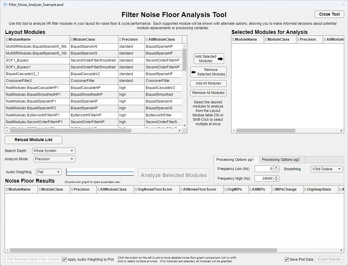
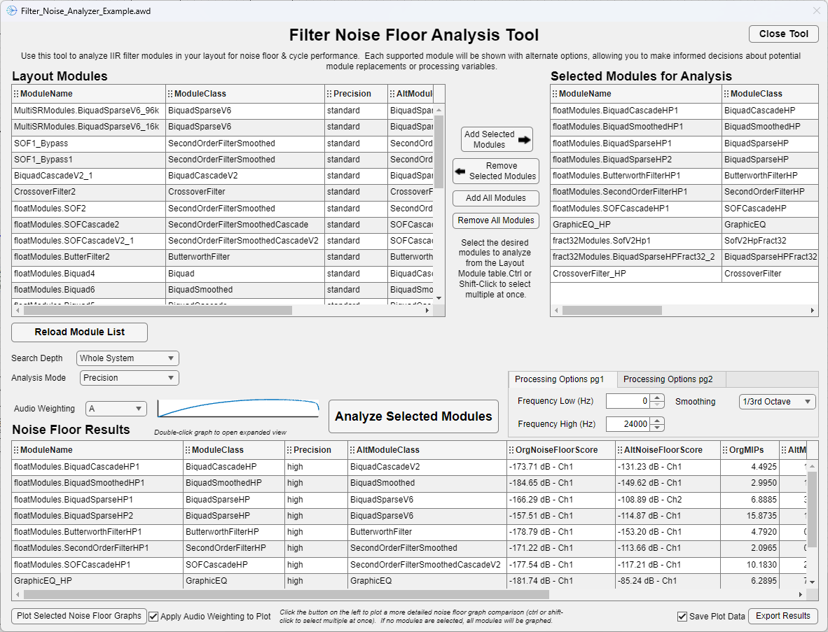
When you open the Filter Noise Analyzer, it should look something like the below image.

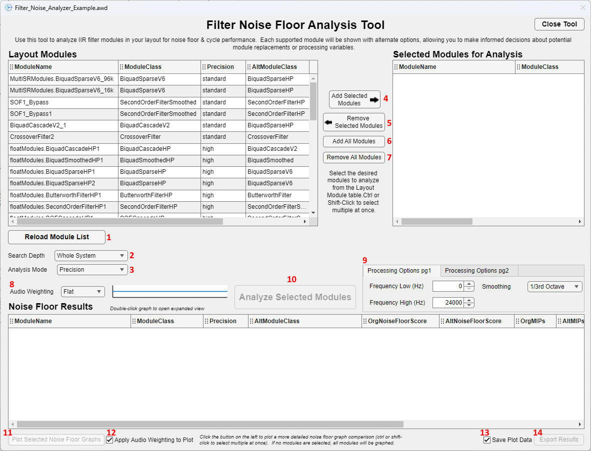
Component Reference Key:

The "Reload Module List" button reloads the module list. It is relevant when the search depth is changed from "Whole System" to "Current Level" and vice versa.
The "Search Depth" drop down changes the search depth of the Tool. "Whole System" will display every filter module in the entire layout, while "Current Level" will only display the filter modules in the page that is shown in AWE Designer.
The "Analysis Mode" mode drop down changes from analyzing the difference between standard and high precision modules, to analyzing the differences between biquad forms.
1. When comparing modules that are using floating point precision, the difference between standard and high precision processing is not a data type difference, but rather a processing method difference. Both processing methods are using the same bit width for their variables.
2. When comparing modules that are using fract32 precision, the difference between standard and high precision processing is usage of an accumulator with a larger width.
The "Add Selected Modules" button adds highlighted modules from the Layout Module Table (left side) to the Selected Module Table (right side).
1. You can select multiple modules by control clicking on each one. You can quickly select multiple modules in a row by clicking on the first relevant module, and then shift-clicking on the last relevant module.
The "Remove Selected Modules" button removes highlighted modules from the Selected Module Table (right side) and puts them back onto the Layout Module Table (left side).
The "Add All Modules" button adds all modules from the Layout Module Table (left side) and moves them to the Selected Module Table (right side).
The "Remove All Modules" button removes all modules from the Selected Module Table and moves them to the Layout Module Table (left side).
The "Audio Weighting" drop down changes the weighting applied to the noise floor calculation. The magnitude response of the chosen weighting is shown next to the drop down.
Various processing options can be changed in these two pages
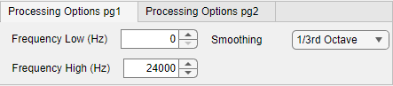
1. The Frequency Low/High values set over what frequency range you want to analyze the filter noise floor. While the default values are 0 to half the sampling rate (nyquist) of the input and output pins of the layout, there is no limit imposed on the high frequency value. This might be useful if the specific filter module is operating at a higher sample rate than the input and output pins. Please note that these values affect the calculated output score, but does not affect the plot that can be displayed. The plot will always display the full frequency spectrum from 10 Hz to Nyquist.
2. The Smoothing drop down lets you choose a smoothing amount for the noise floor calculation and plotting. This is actually incorporated into the resulting score value. 1/3rd Octave Smoothing is selected by default.
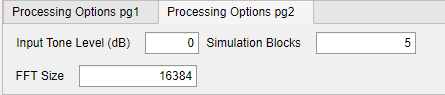
3. The Input Tone Level value is the level (in dB) that the input tone is set to.
4. The FFT Size value sets the size for the FFT analysis when calculating the noise floor.
5. Simulation Blocks changes the amount of samples processed when calculating the noise floor. The higher the number, the longer each calculation takes.
The "Analyze Selected Modules" button will perform the noise floor analysis on the selected modules in the Selected Modules Table and display the results in the bottom Results Table.
The "Plot Selected Noise Floor Graphs" will plot the magnitude response of the noise floor in a new figure window for each selected module in the Results Table.
1. You can select multiple modules with ctrl + click and shift + click.
2. If no modules are selected, it will graph every module. Alternatively, you can select every module with ctrl + A.
The "Apply Audio Weighting to Plot" checkbox will change whether the plot for the detailed noise floor has the selected Audio Weighting curve applied to the output plot or not.
The "Save Plot Data" checkbox will control whether or not the plot data for the magnitude responses are saved as well.
The "Export Results" button will open up a GUI to export the data in the Results Table to a .csv or .xlsx file.
1. It will add, based on the instance id, the processor type information (which is NOT shown in the Results Table).

Tutorial

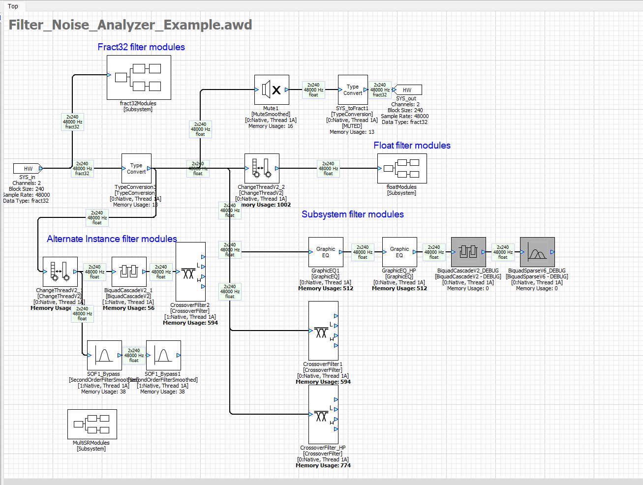
In order to go through this tutorial you will need the Filter_Noise_Analyzer_Example.awd found in the Examples folder. When you open the layout, it should look like this:

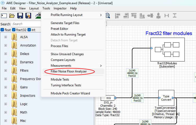
From here, open the Filter Noise Analyzer from the tools menu (circled in red below):

And then you should be able to see the tool open up (which you might notice is the same as the first image up top):

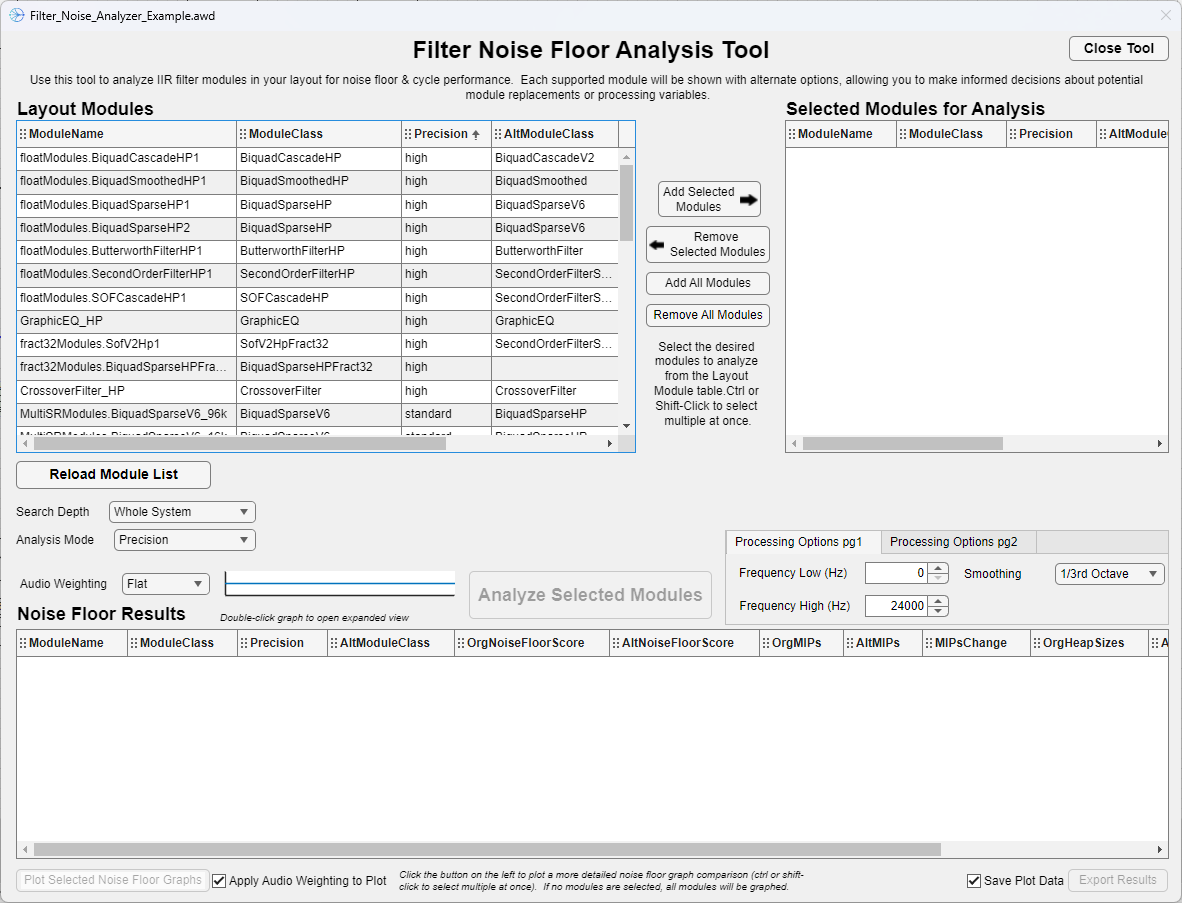
You might notice every single module in the layout is shown. By default, it loads in "Whole System" search depth. You can sort the list by any of the column names. Let's look for all of the high precision modules to analyze. Move the mouse over the "Precision" column name and click the two arrows that show to sort the table by precision (it will look like this: ). After this, the table should look like this:

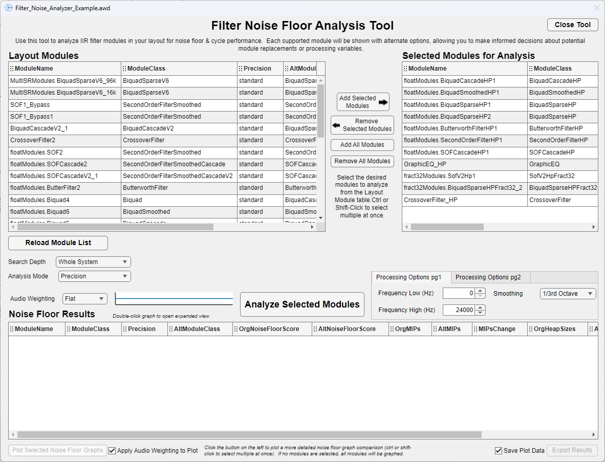
Click on the first row, and then hold shift and click the last high precision module (CrossoverFilter_HP). It should highlight all of the modules in between as well. Next, click "Add Selected Modules" to move those selected modules to the table on the right. It should look like this after they are moved:

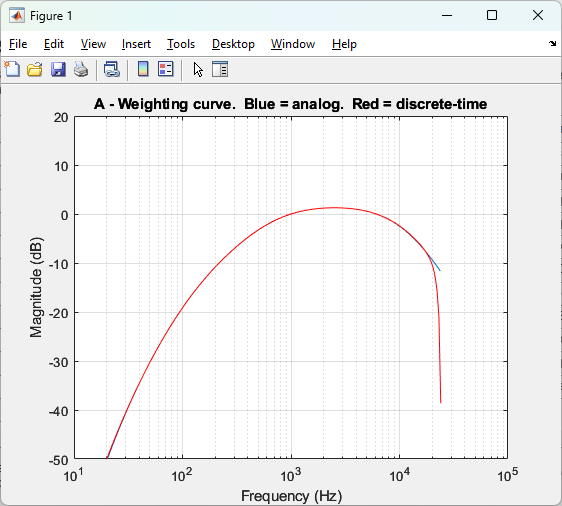
You will notice the "Analyze Selected Modules" button is now enabled. Before we analyze the modules, however, let's change some options. Let's change the "Audio Weighting" drop down from "Flat" to "A" weighting. You should notice the graph next to it change from a straight line to the magnitude response of the A-weighting curve. If you want to look at the curve closer, you can double click the graph to open a detailed graph that should look like this:

Now let's press the "Analyze Selected Modules" button. After a few moments, the tool should be displaying results like so:

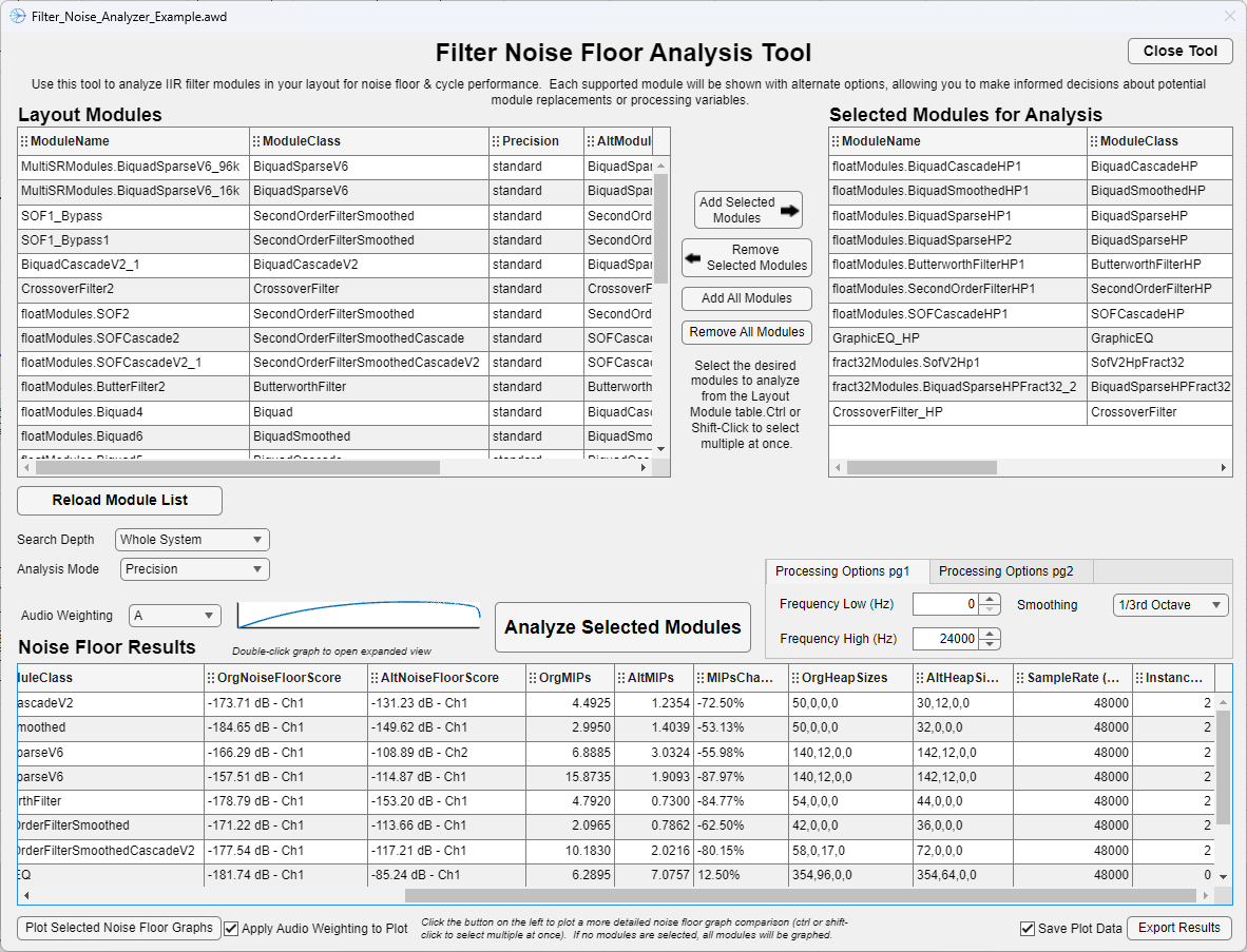
If you scroll the horizontal bar to the right, you should be able to see more data:

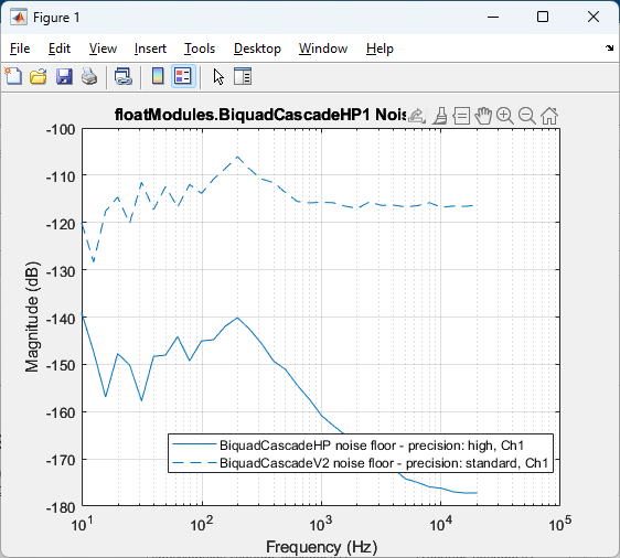
Let's go through the results of the first row, the one titled floatModules.BiquadCascadeHP1.

ModuleName
- This is the unique name of the module as defined in the layout.
ModuleClass
- This is the class of the module that is being instantiated.
Precision
- This is the precision of the module in the layout, either "Standard" or "High".
AltModuleClass
- This is the class of the alternate module that is being used to compare for the alternate precision type. So in our case, the "Standard" precision version of the BiquadCascadeHP module class is BiquadCascadeV2.
NoiseFloorScore
- This is the dB score of the noise floor of the module in the layout. A lower value is a better noise floor. Most of the time, the "High" version of the module should have a lower score than the "Standard" version.
- This value is the max noise floor value of the worst channel.
AltNoiseFloorScore
- This is the dB score of the noise floor of the alternate module to the listed one, that is, a module of the AltModuleClass but with the same variables and arguments of the original one. So in our case, this score corresponds to the noise floor score of a BiquadCascadeV2 module with the same coeffiicents.
MIPs
- This is the MIPs (performance metric) of the original module in the layout.
- Please note that if you are in native mode, the absolute measurement can vary from run to run. If you press the "Analyze Selected Modules" button multiple times, the exact value will most likely not be the same.
AltMIPs
- This is the MIPs of the alternate module.
MIPsChange
- This is the percentage change of the MIPs required to process the module if you changed it to it's corresponding type. A negative value means a reduction in processing power. So in our case, the -79.60% means that if we changed our module from BiquadCascadeHP to BiquadCascadeV2 we would save 79.60% in processing power.
HeapSizes
- This is the memory allocated from the heap for the module in the layout. The four numbers correspond to the FastA, FastB, Slow, and Shared heaps.
AltHeapSizes
- This is the memory allocated from the heap for the alternate module in the layout. The four numbers correspond to the FastA, FastB, Slow, and Shared heaps.
Sample Rate (Hz)
- This is the sample rate of the module in Hertz. The tool can analyze modules in different sample rates (although be wary of the frequency range settings).
InstanceID
- This is the Instance that the module is instantiated on. When doing the noise floor analysis, the module and it's corresponding module are both processed on the targeted instance.

The next thing to do is to plot the detailed noise floor graph. Click the first row and then hit the "Plot Selected Noise Floor Graphs." A plot should come up that looks like this:

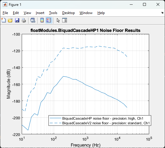
As you can see by the legend, the noise floor of the high precision version of the module is significantly lower than the standard version of the module. Through this figure, you can choose to save this as an image file if desired. Let's try plotting it without the audio weighting applied, just to see what it looks like. Uncheck the "Apply Audio Weighting to Plot" checkbox and click the "Plot Selected Noise Floor Graphs" once again. It should now look like this:

You can see here that the energy especially at the lower frequencies is higher, revealing the effect the audio weighting had on the data. Note that you cannot change the results of the data without reanalyzing, just what the graph looks like. If you select multiple modules, it will display a separate graph for each module.

Certain modules will graph more if there are different "sets" of coefficients to compare, such as the CrossoverFilter and the BiquadSparseHP. Let's graph those two to see what they look like.

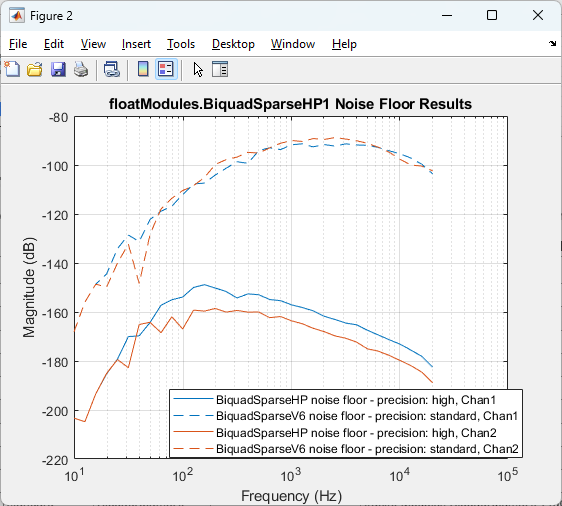
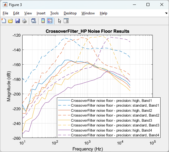
You can see in these images the different sets of filters being compared (different bands for the Crossover Filter and different channels for the Biquad Sparse Filter). Please note once again that changing the frequency range doesn't affect what shows up in these plots, only the noise floor score.

The last thing in our tutorial is to export the data. Click the "Export Results" button. It should pop up a GUI to save the data. Give it whatever filename you want and then open up the resulting file. As you examine it, it should match up with every entry in the table except that there is one additional data point - ProcessorType. This should correspond with the particular instance that the module is instantiated on. There will also be the data to plot the detailed noise floors, both weighted and unweighted (if the checkbox was checked). If you saved as a CSV it will be in a separate file. If you saved as an XLSX it will be on a separate sheet.

And that's it! You can repeat a similar process to this one to see the noise floor differences when comparing biquad forms, DF2, DF1, and TDF2. Simply change the "Analysis Mode" drop down to biquad form and repeat the steps.

How the Noise Floor is Calculated

Users of this tool may wonder how we are calculating a singular "noise floor score" value given that each module may have multiple channels, sets of coefficients, among other things. When thinking about the noise floor of a module, we generally are interested in the worst case scenario. So to do this, we will generate a multi-sinusoidal signal as an input. The frequencies of this sinusoid are then set to be equal to the poles of each modules' biquad coefficients. Next, we analyze the noise floor of the output signal as processed through the filter module. We are looking for the energy present in the signal, excluding the frequency bins that match the frequencies of the input sinusoid in order to get the noise floor.

Generating the Input

Find all pole locations of each filter module and derive the angles (frequencies) $w(k)$ of the pole locations $$ w(k), k=1 \dots K $$ where $K$ is the number of poles. $w(k)$ is between $0$ and $\pi$.
Let $L$ be the size of the FFT. Then we define the bin bandwidth $\Delta W$ as: $$ \Delta W = \frac{2\pi}{L} $$
Next, find the frequency index $f_{index}(k)$ of the pole angles. We quantize them to fit exactly in one of the bins in the L-point FFT. $$ f_{index}(k)=\text{round}\left(\frac{w(k)}{\Delta W}\right), k=1 \dots K $$
Generate the multi-sinusoidal input signal $x(n)$ using $\Delta W \cdot f_{index}(k)$ as the frequencies, which fit exactly in one of the frequency bins: $$ x(n)=\sum_{k=1}^{K}\sin\left(\Delta W \cdot f_{index}(k) \cdot n\right) $$

Getting the Noise Floor Score

After processing the multi-sinusoidal signal through the filter module, we calculate the noise floor by analyzing the output signal.

Take a L-point FFT of the output signal, $y(n)$, and compute a power spectrum $$ P(i)=\frac{1}{N} \cdot FFT(y(n))^2 $$ where $P(i)$ is the power at each bin and $i=1 \dots L/2+1$. There is no windowing applied before the FFT is taken because windowing smears the signal power across multiple bins within the main lobe of the window. Without windowing (also known as using a rectangular window), the signal power is found only at the frequency bin $f_{index}(k)$.
Eliminate the signal power by replacing each bin that corresponds with the input frequencies of the sinusoid with the power of the previous bin. Then the resulting power spectrum will contain only the noise floor data: $$ P(f_{index}(k))=P(f_{index}(k)−1), k=1 \dots K $$
Apply the audio weighting to the output and limit the power spectrum to the frequency of interest. This range is a user defined. $$ P_{weighted}(N) = P(N) * H(N), N = {n \in i \mid f_{\min} \le n \le f_{\max}} $$
Lastly, smooth the power spectrum and take the mean to get the final value. If the module is multi-channel, the score is the value of the worst case.
This is mainly important if you have a module that has different coefficients per channel. Otherwise, the channel difference is irrelevant since we have the same input sinusoid on every channel.

Tool Limitations and Notes

Opening the Tool

When first opening the tool, it will attempt to prebuild your layout. If the layout has errors, then it will pop up an error telling you what the message is and then close itself to allow you to fix the prebuild error. This can be avoided by prebuilding yourself before using the tool by pressing the "Propgate Changes" button.

Debug Mode

If your layout is in the "Debug" Build Configuration (set in the Layout Properties Menu), then this tool will discover any modules that are in Debug mode. If they are not, then the tool will not discover them.

Module Support

Not every IIR filter or biquad module is supported. There are few categories that we have intentionally left unsupported:

1. Biquad Modules with Control Pins
2. 24 bit and 16 bit Biquad Modules

Otherwise, we have strived to support the most common and up to date filter modules, but if you think there is one that should be supported that is not, please contact us. It is also possible to have a custom module show up, although it requires additional code and functions to be written. Additionally, there are a few modules that don't have an obvious alternate type and do not support displaying data for the non-existent alternate type, although you can still see the data for the module itself. See below as an example:

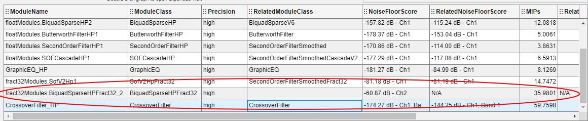
Also, because the noise floor is calculated using poles, if the biquad has no poles (either the biquad is set to be passthrough and/or the coefficients relating to the poles are set to zero), there will be no noise floor result.

In terms of biquad form support, there are only a few modules that actually support different biquad forms, so if you are looking for this type of analysis, please make sure the modules you are using support different biquad forms.

Module Modifications

When using the tool, there is no way to change module variables or arguments. The tool currently takes a snapshot of the current layout when you open it and is unable to accommodate any changes made while it is open. The best way to get the tool to apply any changes is to close it, make the changes that you want, and then reopen the tool.