AWE Architecture Document

Introduction

Audio Weaver is a development platform for audio product developers. It contains a graphical editor (Designer) that is used to configure run-time libraries of audio processing functions (AWECore). This document provides an overall description of Audio Weaver's architecture and is a good starting point for anyone new to the technology. This guide covers general Audio Weaver principles and is applicable to a range of processors from microcontrollers, through DSP's, and all the way to multicore SOCs. These principles apply across processors, but the specific implementation may vary depending on the details of particular systems or implementations.

The high-level architecture of Audio Weaver is shown in Figure 1 below. Audio Weaver Designer is the primary interface. Designer is built upon a foundation of MATLAB scripts. MATLAB is used for automation, scripting, and parameter calculations. The "Server" is a Windows program that has 2 functions:

1. Contains an internal Windows run-time target that performs real-time simulations.

2. Manages communication between the PC and the embedded target.

The Server communicates to the target via the "tuning interface". This could be Ethernet, USB, UART, or SPI depending on the peripherals available on the target.

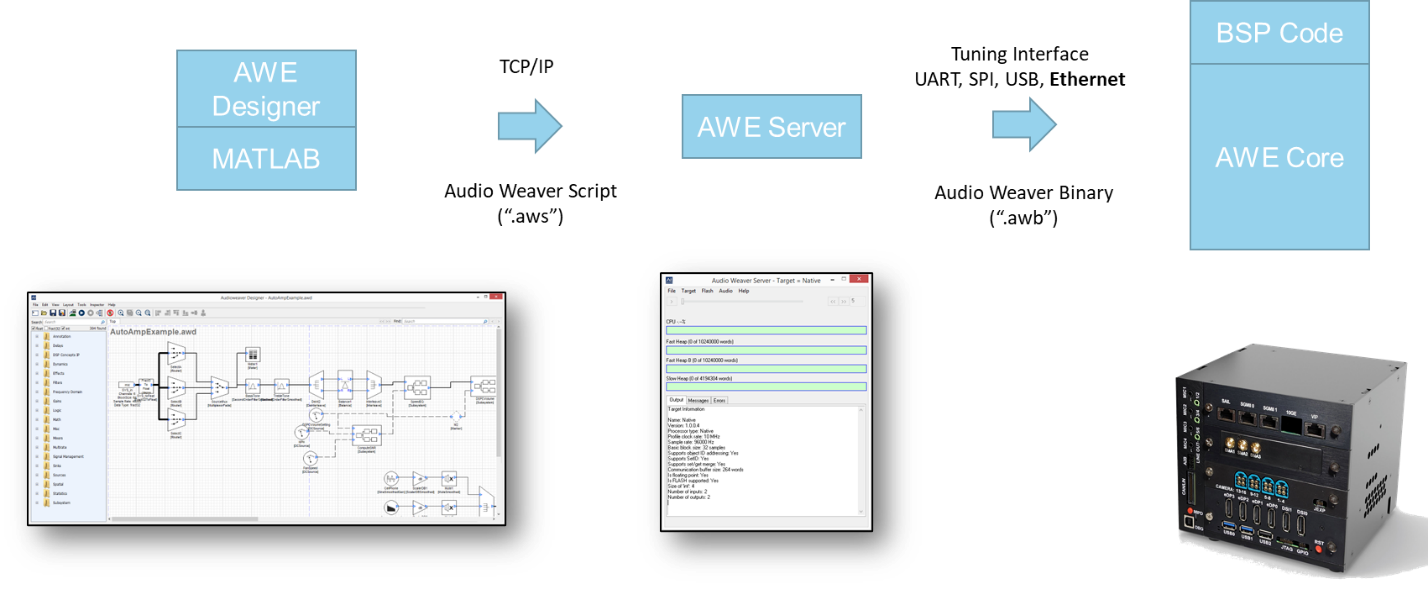
Figure . High-level Audio Weaver architecture showing the various components and how they communicate.

The embedded target contains a board support package (BSP) which manages real-time I/O and the tuning interface. The BSP feeds blocks of audio data to AWECore for processing. The BSP is usually custom written for each target. AWECore libraries are available for the instruction sets shown in Figure 2 and we continue to add new instruction sets to meet market demand. The code is highly optimized and designed for efficient real-time execution.

Arm: Cortex-M4, Cortex-M7, Cortex-M33, Cortex-M55, Cortex-A

Tensilica: HiFi-2, HiFi-3, HiFi-4, HiFi-5, HiFi-Mini

Qualcomm: Hexagon including HVX, Kalimba

Intel and AMD: x86, x64

Analog Devices: SHARC, SHARC+, SHARC-FX

Texas Instruments: C6x, C7x

CEVA: X2

XMOS: xcore-ai

Figure . Instruction sets supported by Audio Weaver

Designer and MATLAB communicate with the Server over TCP/IP. Text messages are sent using Audio Weaver Script (.aws). This is a human readable text format and is like a netlist. The script describes the overall system including modules used, connections, and parameter settings. The Server translates the script to Audio Weaver Binary (.awb) messages. The binary format contains the same information but is easier to decode on the embedded target.

The term "tuning interface" will be used to describe the connection between the Server and the target processor. Note that the tuning interface and protocol are used to build the system, tune parameters in the lab, and also run-time control in a deployed product.

There are 3 versions of the Designer tools available:

Standard -- Provides access to the graphical interface and does not require a MATLAB license. The Standard version is sufficient for most users building, tuning, and deploying systems.

Pro -- Includes access to the MATLAB scripts. Useful for testing and build automation. Requires a MATLAB license[^1].

Pro + Custom Module SDK -- For engineers creating new modules to be used in Audio Weaver. This includes writing C code or wrapping existing libraries. Requires a MATLAB license.

The document begins with an overview of Audio Weaver and the breadth of features. Then we describe the real-time architecture used for audio processing. This includes basic single threaded systems and more sophisticated multithreaded and multicore systems. Then we discuss modules, their underlying architecture, and how they fit into the run-time framework. Next, we discuss how to control processing in products. We give a brief overview of the MATLAB automation API and lastly discuss how Audio Weaver run-time libraries are incorporated into products.

Audio Weaver Basics

Designer is a PC tool for creating and tuning signal flows. The main window is shown in Figure 3 with several key areas highlighted. The Module Browser is where you find modules and then drag them onto the Canvas. You then use Inspectors and the Property Editor to change parameters.

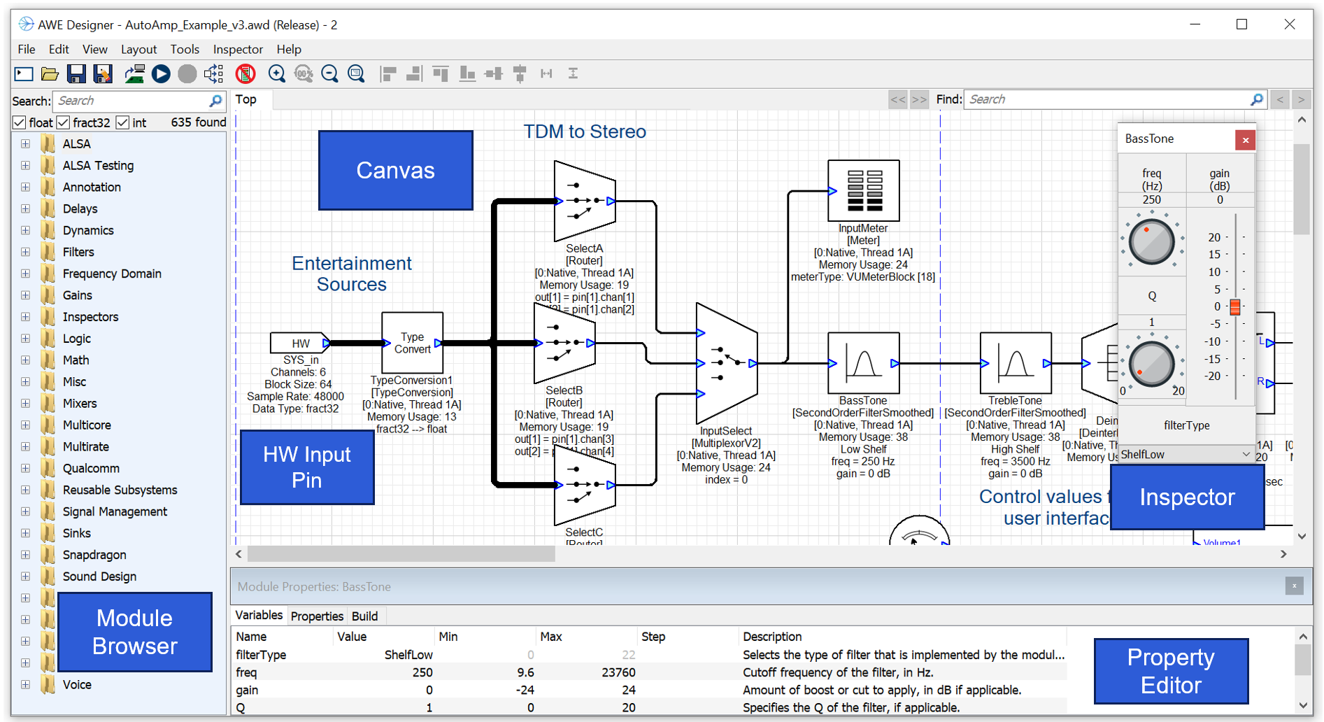
Figure Main Audio Weaver Designer window.

Designer

Hardware Input and Output Pins

Audio arrives into the system on the HW Input Pin. In the example shown above, this is 6 channels of audio at 48 kHz with a block size of 64 samples. The audio arrives as fixed-point data (fract32) and is converted to floating-point by the TypeConvert module. Audio Weaver currently supports one HW Input Pin and one HW Output Pin, and all I/O is funneled through these interfaces. The Designer GUI allows you to configure properties of the HW Input Pin while the properties of the HW Output Pin are inherited from the upstream modules.

Modules and Wires

The signal flow is composed of Audio Modules and the connections are called Wires. Each wire corresponds to a buffer of data in memory, and these buffers are reused when no longer needed. This reduces the total memory needed for a system. Audio Weaver stores audio samples in an interleaved format and modules are designed to operate on interleaved data.

Design and Tuning Modes

When you first launch Designer, it is in Design Mode. Here you can update the signal flow, add and delete modules, and change wire information. When you are ready to listen, hit the Build button on the toolbar. The system is built, real-time audio starts, and Designer enters Tuning Mode. In tuning mode, parameter changes are sent to the target and you can hear the changes instantly. Tuning mode also supports profiling, and visualization of signals (Meters and Sink inspectors).

Native PC Simulation

Audio Weaver supports real-time audio processing on the PC. This is called the Native PC Target and allows development to happen independent of target hardware. The PC makes an ideal development environment with a very powerful processor, large memory resources, and a variety of audio devices. Audio Weaver supports real-time audio through DirectX or ASIO I/O. Many customers leverage off-the-shelf sound cards for these types of simulations. DSP Concepts also separately sells rapid prototyping hardware which combines line level I/O with microphones. All I/O is synchronized allowing echo cancelers and other voice processing to run smoothly. The DSP Concepts RAPD Kit is shown in Figure 4.

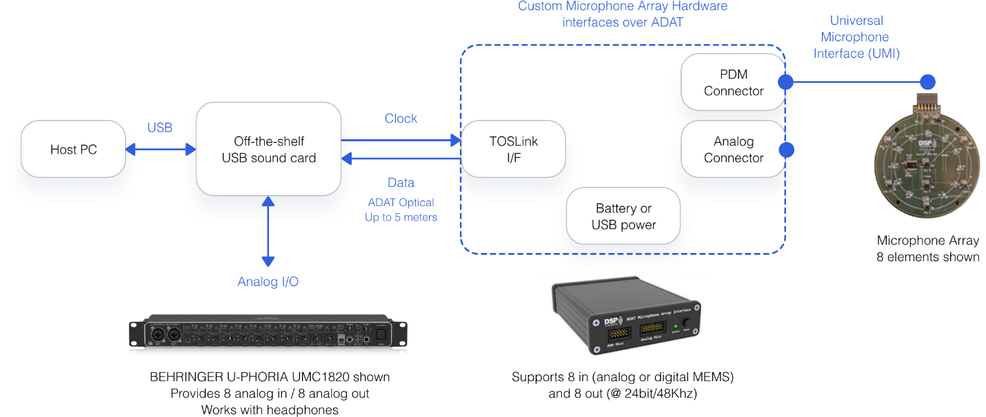
Figure . DSP Concepts RAPD Kit provides synchronized audio I/O for Native PC simulation.

80 to 90% of Audio Weaver development happens on the PC independent of target hardware. In Native PC Mode, you can create and tune signal flows, integrate new modules, perform A/B listening tests, and develop regression tests. Running on target hardware is used to verify resource consumption and to interface to the actual peripherals used.

Attaching to a Running Target

Audio Weaver is also able to attach to a running system without disturbing the audio processing. This is similar to attaching a debugger to a running processor. It allows you to examine system state without reloading and restarting the system. Refer to Attach to Running Target in the Audio Weaver Designer User's Guide for more information on this feature.

Inspectors

Examples of inspectors are shown in Figure 5. Audio Weaver provides a base set of GUI widgets (knobs, sliders, drop lists, meters, etc.) that you can use when developing custom inspectors. Inspectors are available in both Design and Tuning Modes.

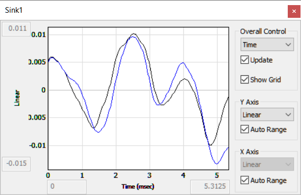
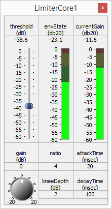
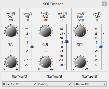
Figure . Examples of some inspectors that are available in Audio Weaver.

Hierarchy

Audio Weaver supports hierarchy via the subsystem module. This allows you to organize your signal flow by placing specific functions into their own subsystems. Audio Weaver supports arbitrary levels of nesting and you can places subsystems, within subsystems, and so forth. You can also visually create custom subsystem inspectors using the Inspector Designer, and then use this to tune your subsystem. It is easy to create reusable subsystems and share them with your team members.

Profiling Resource Consumption

Audio Weaver provides multiple methods of profiling your design to determine resource consumption. These are illustrated in Figure 6. By default, the Server window shows aggregate information when in Tuning mode. Designer can go a step further and provide detailed module-by-module information. And finally, if you are concerned about variations in CPU load, you can use the Peak Profiling feature to identify issues.

(A) Aggregate profiling shown on the Server.

(B) Per module profiling.

(C) Peak profiling.

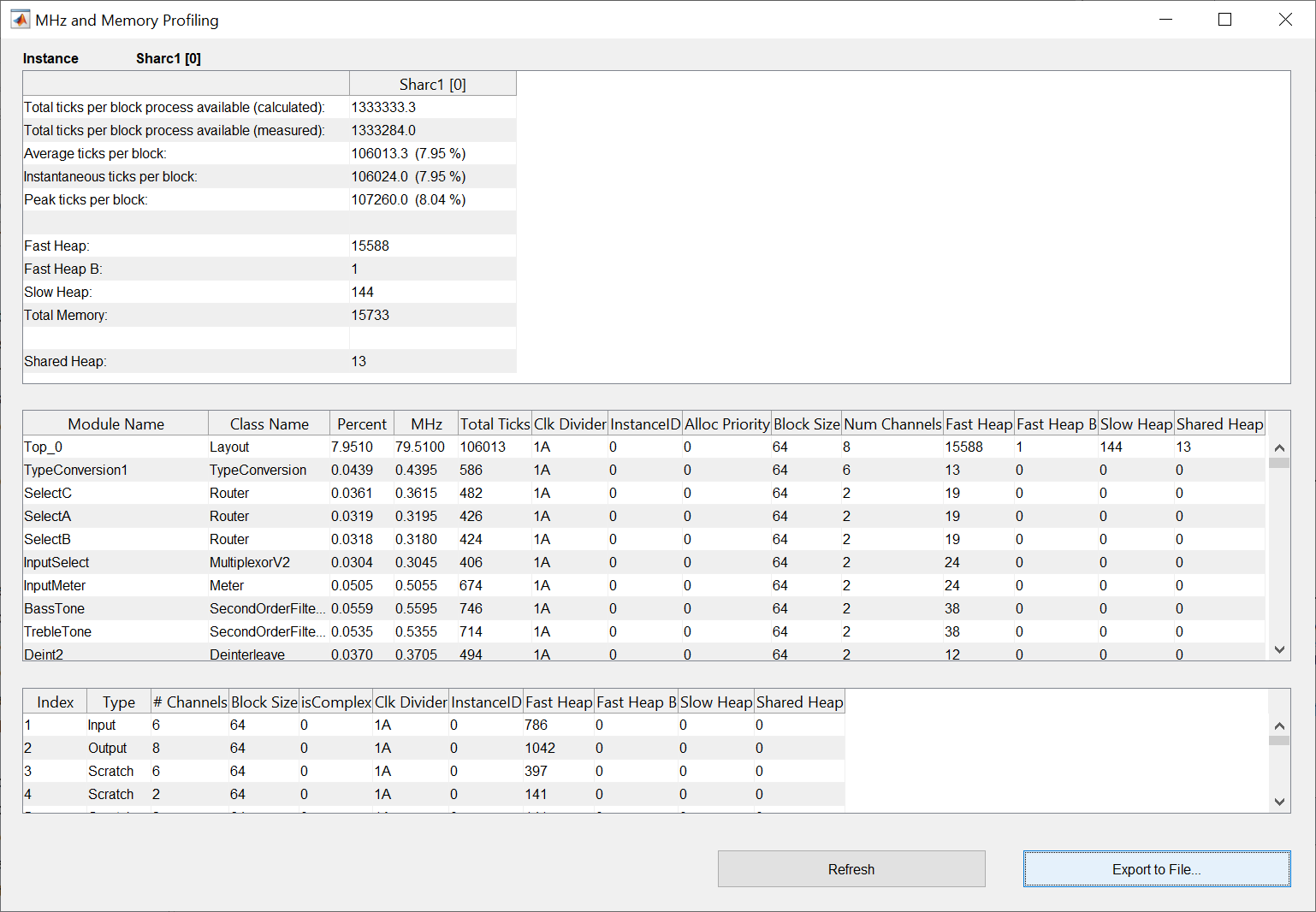
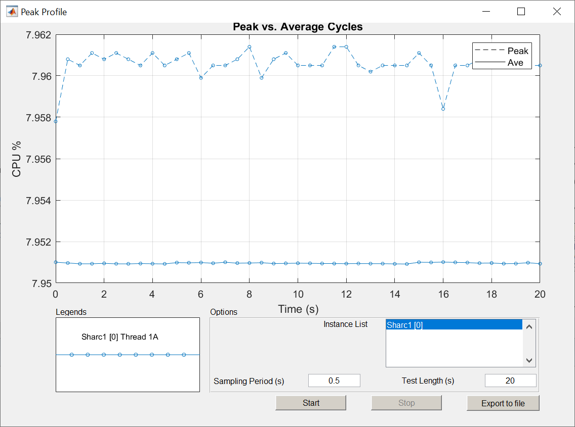
Figure . Multiple methods of profiling in Audio Weaver. (a) Aggregate information on the Server window. (b) Detailed per module information. (c) Peak profiling showing variation over time.

Advanced Signal Flow Design

Audio Weaver has a wire buffer format which provides a high degree of design flexibility. Each wire buffer locally encodes the number of channels, block size, and sample rate. With this you can:

• Define multichannel signals holding from 1 to 1023 channels. Processing 5.1, 7.1, or 7.1.4 signals is straightforward.

• Mix processing at different sample rates. For example, playback processing can be run at 48 kHz while voice processing is at 16 kHz.

• Control rate processing can be done at a decimated rate to reduce CPU consumption.

• Multithreading allows you to mix block sizes and execute processing at different thread priorities.

• Multicore processing allows you to seamlessly partition processing across multiple cores in an SOC.

You can use these features to optimize your signal flow and reduce the CPU load. In general,

• Larger block sizes are more efficient than smaller block sizes.

• Using an N-channel representation is better than processing N mono channels.

• Processing at a lower sample rate, or decimated rate, is more efficient.

Your signal flow can also incorporate feedback. Feedback occurs on a block basis and is useful, for example, when generating reference signals for an echo canceller, or designing reverb effects.

Section 3 provides more details on Audio Weaver's real-time architecture.

Target Information

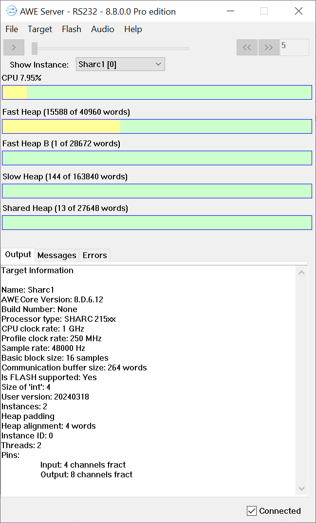
Information about the currently connected target is shown on the Server window as illustrated in Figure 7. You can switch between targets using the "TargetChange Connection" menu of the Server.

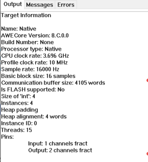
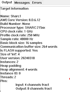
Figure . Target information shown on the Server. The window on the left corresponds to Native Mode when the audio processing is performed on the PC. The right side is when connected to a SHARC 21594 EZ-KIT.

File Formats

Audio Weaver stores your signal flow using two different file formats:

.awd -- binary format used natively by MATLAB

.awj -- json text format

You select which format to use when saving a design. We recommend that you use the AWJ format because the files are smaller, compatible with source code repositories, and easier to compare.

Advanced Tools

Audio Weaver has additional tools which are useful in the product development process. We touch briefly on them here and more details can be found at the online Documentation Hub.

Batch File Processing

In Native mode, you can quickly process WAV files through your design. The processing is faster than real-time and is useful for batch processing of large datasets. You access this through the Designer "ToolsProcess Files" menu item.

Tuning Interface Test

This is useful for software developers integrating the AWECore libraries on new hardware. The regression test is accessed through the Designer "ToolsTuning Interface Tests" menu item. The tests measure the robustness and speed of the tuning interface.

Computing Frequency Responses

If your module is linear and time invariant (i.e, a "filter") then Designer is able to compute its frequency response. Right-click on the module in the canvas and select "Plot Frequency Response". An example is shown below.

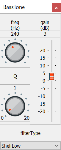
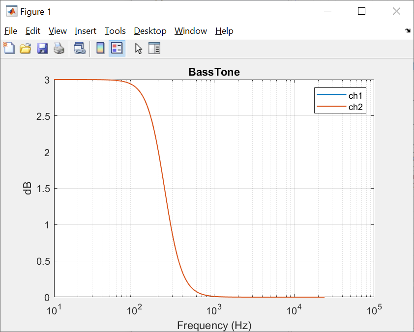
Figure . Frequency response for a second order filter configured as a low-shelf.

Designer is able to compute the frequency response between two locations in the signal flow. Add Marker Modules to the wires you want to measure between, and then use the "ToolsMeasure Frequency Response" feature of Designer. An example is shown below.

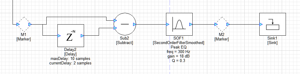
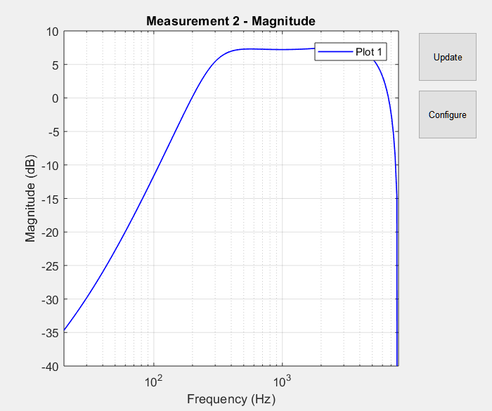
Figure . Point to point frequency response measurements are made between two Marker modules in the Designer Canvas. In this example, the measurement is made between Markers M1 and M2.

Diffing Systems

Audio Weaver contains tools for comparing two systems. The "ToolsShow Unsaved Changes" menu item displays what changes were made since the file was opened. This is useful to see what variables were updated during a tuning session. You can also compare two different designs using the "ToolsCompare Layouts" feature. In both cases, Audio Weaver generates a text "list file" containing parameter values and wiring information and then uses an external diffing tool to show what changed. An example is shown below.

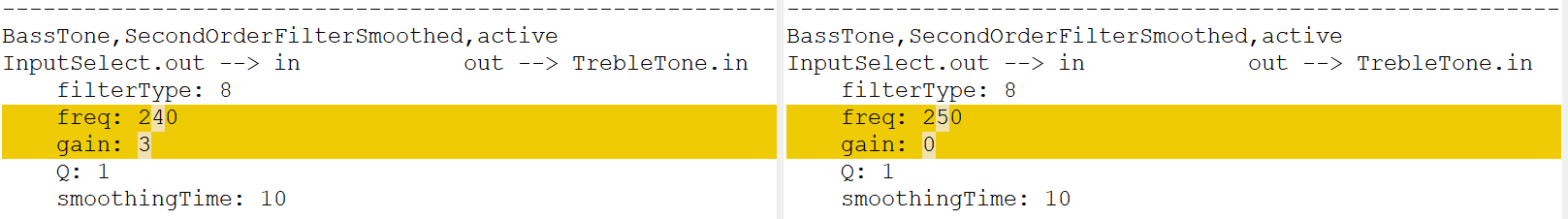
Figure . Example showing the text list format file and how changes can be found using standard diffing tools.

Debug and Release Builds

Audio Weaver has a feature which allows you to selectively include / exclude modules. Modules in the signal flow can be marked as being "Debug" or "Release". Release is the default when you first drag a module to the canvas. You can then configure Designer to do a "Release" or "Debug" build. In a Debug build, all modules in the design are included. In a Release build, all modules marked as Debug are removed. In practice, you may add extra Meter and Sink modules to your design for debugging and then exclude these from the Release build.

Channel Names

Audio Weaver allows you to add names to the channels in your design. To get started, right-click on a wire and select "Edit Channel Names". Name information is then propagated throughout and displayed on level meters and multichannel controls. An example is shown below. For more information, search for "Channel Names" on the Documentation Hub.

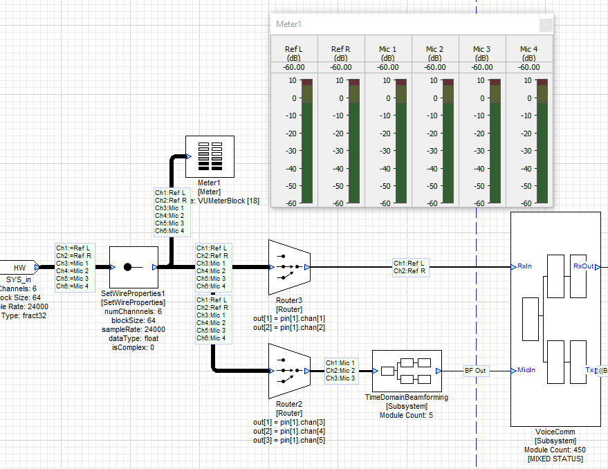
Figure . Example of channel names used in the Designer GUI.

Channel Latency

In many audio applications, it is important to maintain alignment of audio channels throughout the signal flow. Audio Weaver can be setup to track and report latency. The feature is similar to channel names and an example is shown below.

Figure . Example showing latency tracking in the Designer GUI.

Module Libraries

Audio Modules are organized into Module Libraries in Audio Weaver. Each module library is contained in its own Windows DLL, and the DLL is loaded when the Server launches[^2]. You can list all available modules using the "TargetList Modules" menu of the Server. An example is shown in Figure 13. Audio Weaver has 100's of modules available, sufficient for most audio use cases.

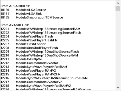
Figure . The Server can show what modules are available for you to use. The modules are grouped into DLLs and this is only a partial list of the first two libraries.

In total, Audio Weaver contains over 500 different processing modules organized into separate module libraries.

Standard -- Time domain playback processing

Advanced -- Multirate and frequency domain processing. Also multichannel versions of some modules.

Voice -- Echo cancelers, beamformers, and noise reduction for voice applications

Sound Synthesis -- PCM generators for chimes, AVAS, and sound design applications

Machine Learning -- ML run-time interpreters (TFLM and ONNX). Feature extraction.

These modules are sufficient for most playback and voice processing use cases and many customers are able to develop their products using the supplied modules. More details are found on the Documentation Hub in the Section entitled Module Users Guide.

You can add or remove module libraries in Designer via the "FileSet Module Path" menu. This opens the dialog shown below. If you are developing custom modules, you must add your custom libraries here. When you close this window, Designer rescans all module libraries and updates the Module Browser.

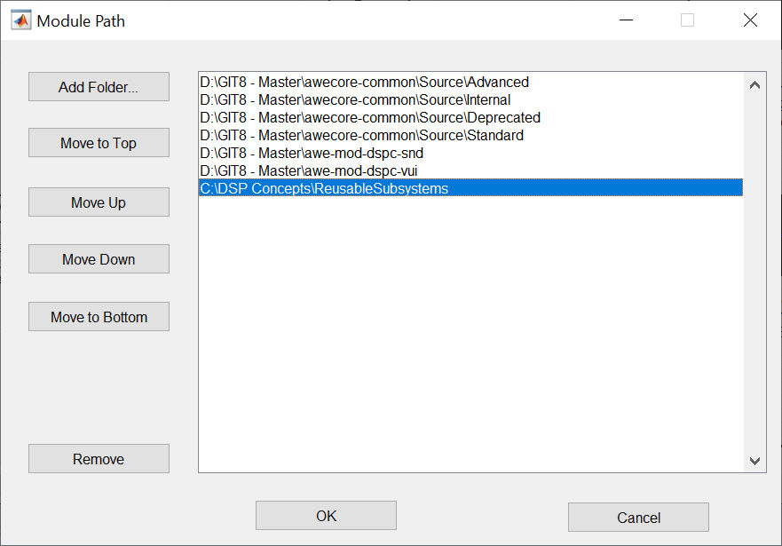
Figure . Window to configure the module search path.

Custom Module API

You can also add custom modules through our Custom Module API. This is for advanced users and IP partners who want to leverage existing audio processing functions within the Audio Weaver execution environment. Modules are developed using a combination of MATLAB code and C code. The Audio Weaver Designer includes a Custom Module Wizard which simplifies the overall development process.

Only the module writer needs access to a MATLAB license. Once a module is complete, it can be delivered as an Interpreted Module that is compatible with the Standard Edition of Audio Weaver. The users of the custom module do not require MATLAB licenses.

If you develop custom modules, we recommend that you start on Windows and debug your module in Native mode. This is the friendliest development environment and easiest to debug. Once your module is working in Native mode, and you have a regression test, then migrate to an embedded target. Recompile your code and verify that it is working. Then profile to check the resource consumption and see if it requires optimization. We recommend keeping the Native and target implementations in sync (same sound quality) so that Native mode can continue to be used for prototyping, tuning, and testing.

Open IP

DSP Concepts provides access to signal flows implementing a variety of useful audio features. These signal flows are provided as open Audio Weaver designs allowing you to understand, modify, and tune the IP yourself. We encourage customers to build upon our designs and make improvements for their unique requirements. The designs are found on the Documentation Hub and include:

Presence Detection -- ultrasonic motion-activated on/off control

Direction of Arrival -- Accurate estimation of audio source direction using 2+ microphones.

Bone Conduction Fusion -- For earbuds. Combines a standard microphone with an accelerometer to clean up voice.

PlayWide -- Stereo image enhancement. Widens the perceived sound field of stereo playback systems.

PlayBass -- Bass enhancement. Extends perceived bass response by adding harmonics based on low frequency fundamentals.

PlayLevel -- Volume management. Maintains output at a target loudness level despite varying input levels.

PlayVoice -- Dialog boost. Emphasizes the voice band range while attenuating non-voice band signals.

Room Correction -- Automatically applies low frequency EQ to adjust for room acoustics. Compensates for device placement.

Wind Noise Reduction -- Suppresses characteristic noise in specific frequency bands. Requires 2 or more microphones.

Dynamic Instantiation

When a system is built in Audio Weaver, the Designer tool sends a list of commands to the target to instantiate, configure, and connect modules. This set of commands is similar to a netlist and allows you to reconfigure the processing without having to rebuild code. This leads to an agile workflow and avoids having to generate code and rebuild the target image. We refer to this as Dynamic Instantiation.

MATLAB Automation API

Audio Weaver is tightly integrated with MATLAB and you can use MATLAB scripts for general automation, regression testing, and creating custom inspector control panels. Refer to the MATLAB Automation API in Section 6

Flash File System

Some deeply embedded processors, like microcontrollers or DSPs do not have an operating system with a file system. As an alternative, Audio Weaver includes an optional Flash File System which provides basic functionality. The Flash File System is used to store AWB files which are loaded at initialization or WAV file samples for sound generation modules. Modules leveraging this feature include "FFS" in their module class name.

Configuring Audio Weaver

The underlying functionality of Audio Weaver can be configured in several different ways.

Global Preferences

Global Designer settings are accessed file the "FileGlobal Preferences" menu. Some things you can change here are:

• Configure a remote tuning proxy

• Change general Designer attributes like what format to use when displaying delay information

• Configure the module browser

• Set a diff tool

• Change the default audio file used in Native mode

Layout Settings

You can configure settings which apply only to a particular signal flow on the "LayoutLayout Properties" menu item. Here you can:

• See which module classes are used in your design, and the total module count.

• Switch between sound card and file input.

• Enable recording of the hardware output pin in Native mode.

• Switch between Release and Debug builds.

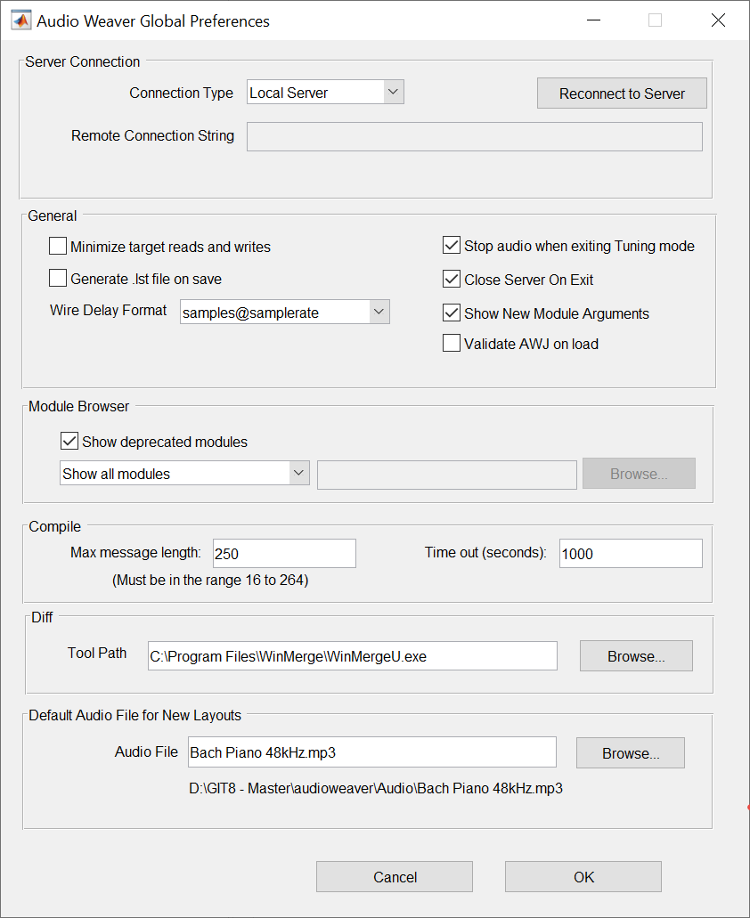
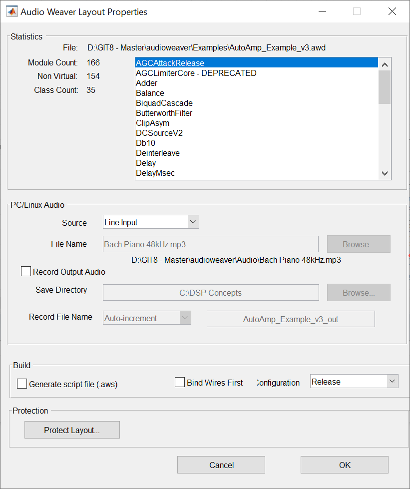
Figure . Designer's Global Preferences and Layout Properties dialog boxes.

Server Settings

The Server has two configuration windows which are frequently used.

Changing the Connected Target

The "TargetChange Connection" menu allows you to change the tuning interface and configure settings.

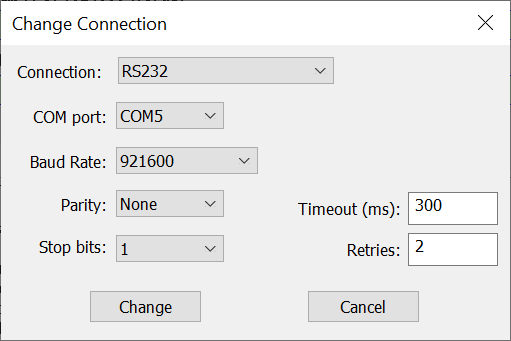
Figure Changing the tuning interface through the Server. Here are the settings for an RS232 connection.

PC Sound Card Settings

You change PC sound card settings in the "FileNative Audio Settings" dialog. You can select multiple devices and switch between DirectX and ASIO drivers. The dialog will show audio devices currently available in your system.

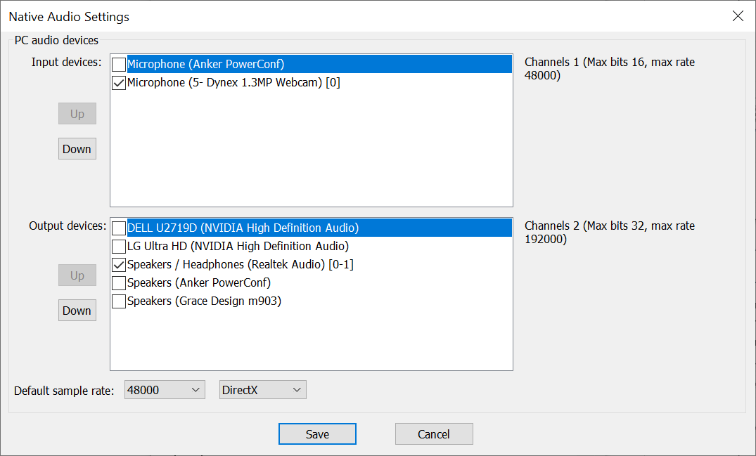
Figure . Configuring audio device using in Native mode through the Server.

Server INI File

The Server stores a larger number of configuration settings in an INI file. The most frequently used INI settings apply to the Native PC target. For easy access, you can get to these directly using the "FilePreferences" window. To access all INI settings, use the "HelpOpen INI File" menu item. This is a text format and uses a standard Key=Value approach. Search the Documentation Hub for "INI File" to learn more.

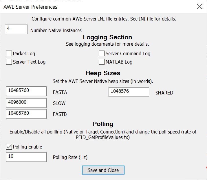
Figure . The Server's Preferences windows allows you to configure a subset of the INI file settings.

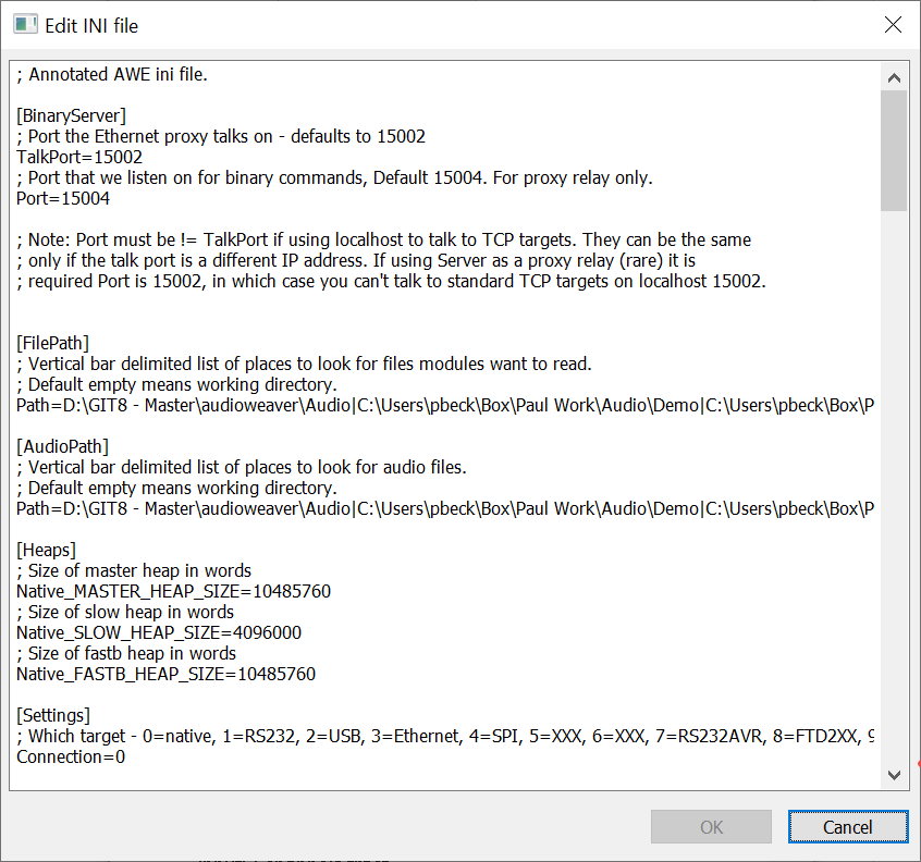
Figure . Partial listing of the Server's INI file settings.

File Search Path

Audio Weaver sometimes needs to access files stored locally on your PC. Instead of using absolute paths (which make it difficult to share designs with others), you can use the File Seach Path feature. You configure this via the "FileSet File Search Path" dialog. In your design, instead of absolute paths, you store only the base file name. Designer then locates the actual file on disk by searching -- in order - through the File Search Path. This feature is mainly used in two places:

1. When specifying an audio file to use in Native mode (Layout Properties dialog).

2. When modules need to access files on disk. Examples are wake word model files or machine learning model files.

Logging Support

You can log data in several different ways in Audio Weaver. The most basic is to record the hardware output pin when in Native PC mode. You configure this on the Layout Properties dialog discussed in Section 2.8.2.

You can also inject and record audio signals inside your signal flow using the WavFileSource and WaveFileSink modules. This feature is available on Native module and on targets that have a file system (like Linux or Android).

The Audio Weaver Server also has built-in logging of messages. This is useful when debugging tuning interfaces or remote tuning proxies. The Server logging information is shown at the top of Figure 18.

Real-Time Audio

Audio Weaver performs block-based audio processing. For each module in the design, the framework calls each module's processing function. For most systems, the larger the block size, the more efficient the processing becomes[^3]. The block size of the system is determined based on what algorithms are running and how much memory is available. A low latency application, like automotive road noise cancellation, might run at a block size of ½ msec. Telephony applications are still latency sensitive, and might use block sizes in the range of 4 msec to 8 msec. Playback applications are less latency sensitive and could use even larger block sizes.

Systems that operate using one block size are single threaded. This is the most basic real-time system. If a system requires multiple block sizes, then multithreading is required. We describe each type in turn.

Single Threaded Processing

Consider the system shown in Figure 20 which operates at a 1 msec block size. This corresponds to 48 samples at 48 kHz. The underlying BSP code will be designed to buffer up 1 msec blocks of audio data, generate an interrupt, and then call the Audio Weaver processing. Real-time audio I/O is usually performed with DMA and double buffering as shown in the figure. The DMA fills (or empties) buffer A while buffer B is used for processing. Every 1 msec the buffers alternate.

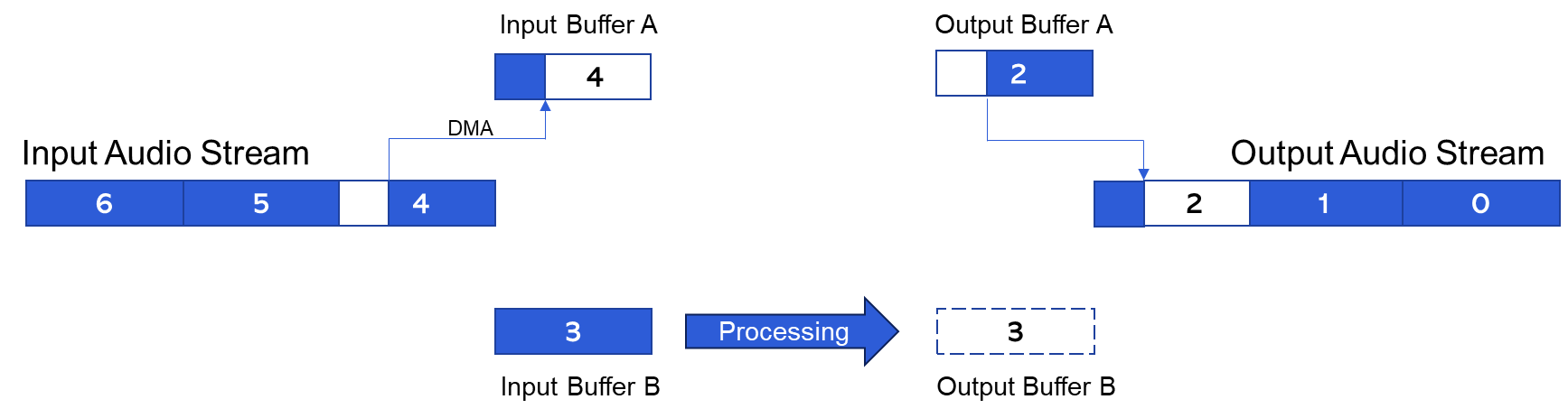
Figure . Single threaded system operating with ping/pong buffers A and B. The numbers correspond to the index of the 1 msec blocks of audio data in the system.

In the system above, you can see that block 4 is filling the input DMA buffer while block 2 is streaming out. The net latency through the system is exactly 2 blocks and this is the lowest latency that can be achieved for a single threaded system. The latency depends on the block size with smaller blocks yielding lower latency.

Basic Block Size

In Audio Weaver, the block size of the DMA operation is called the "basic block size" of the BSP. When the Server attaches to a target, it queries the target and displays information on the Output window. An example for a SHARC 21594 EZKIT target is shown in Figure 7. The basic block size is 16 samples and the sample rate is 48 kHz. The audio processing thus happens every 1/3 of a millisecond.

Wire Buffers

When Audio Weaver builds a system, it determines the execution order of the modules. This routing operation begins at the input pin of the system and proceeds module by module until the output pin is reached. If multiple modules can execute, then heuristics are used to determine which module is next. Consider the simple system shown in Figure 21 which contains hardware input and output pins, and 6 modules.

1. Audio arrives from the BSP on the SYS_in hardware input pin. The data is 32-bit fixed point (fract32), stereo, with a block size of 16 samples.

2. SYS_toFloat converts to a floating-point representation.

3. Scaler1 applies a gain in dB.

4. SOF1 is a Biquad filter with design equations.

5. FIR1 is a 31-point FIR filter.

6. MixerV3_1 is a 2-in / 2-out mixer with a configurable 2x2 mixing matrix.

7. SYS_toFract converts back to fixed-point.

8. SYS_out sends the data to the BSP.

All processing is with stereo data using a block size of 16 samples.

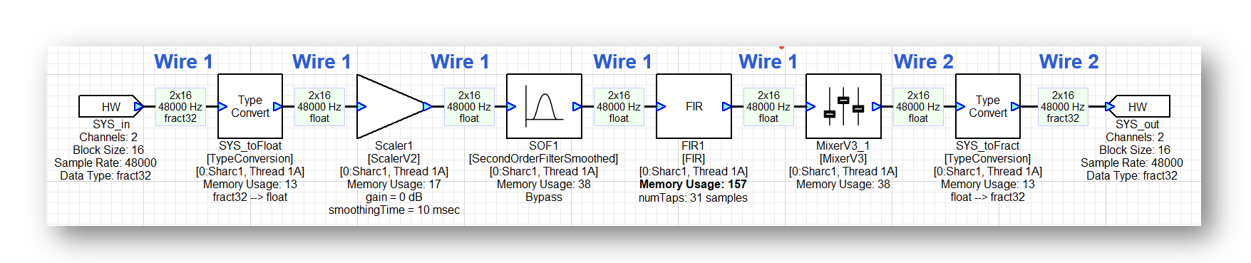
Figure . Simple Audio Weaver system containing 6 modules. On each wire buffer is shown (number of channels) x (block size), sample rate, and data type.

The modules in this simple system execute from left to right as shown in the figure. In Audio Weaver, wire buffers are used to hold intermediate results between modules, and these are marked in Figure 21. Whenever possible, Audio Weaver tries to reuse wire buffers to reduce the total amount of memory required by the system. If a module uses the same wire for input and output, then the processing is in-place. In this example, wire 1 is reused multiple times until we reach the Mixer module. The Mixer module is unable to do in-place processing[^4] and therefore Audio Weaver allocates Wire 2. Wire 2 continues to be used until the output of the system.

Layouts

An ordered list of modules in Audio Weaver is called a layout. The simple system above contains 6 modules in the layout (the HW input and output pins do not count) and the modules are ordered based on their execution order. On the target processor, a layout is presented as an array of N-pointers to module instance structures. When processing audio, Audio Weaver iterates through the modules in the layout and calls the associated processing function for each module. The input and output wires used by each module are preassigned at build time. Execution of a layout is very efficient, and it essentially involves calling the processing function of an ordered list of modules.

The processing of the 6 modules in the layout must be completed within 1/3 of a msec in order for the system to run in real-time. Figure 22 shows activity in different parts of the system. The top-section is the block-based input DMA, the middle-section is the processing, and the bottom-section is the output DMA. The numbers indicate the index of each block. While block 2 is being received, block 1 is being processed, and block 0 is being output.

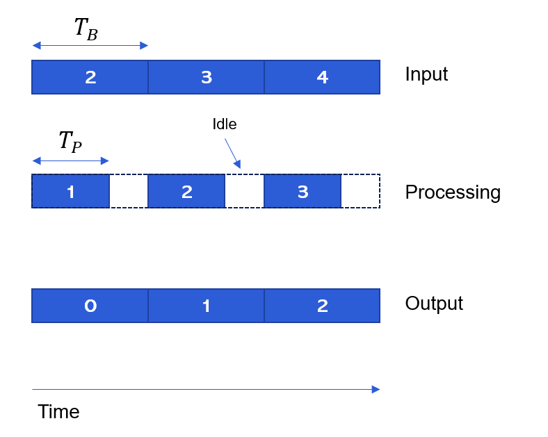
Figure . Single threaded processing over time.

Since the modules all execute within the same layout, there is no added latency. The overall latency of this system is solely due to the I/O, and in this case is 2 x 16 = 32 samples at 48 kHz. Additional latency only occurs if it is explicitly caused by a module. For example, a delay module or an FIR filter with initial coefficients set to zero.

Profiling

Figure 22 also indicates two different times:

\(T_{B}\) = Time between DMA interrupts ("block time")

\(T_{P}\) = Time for the processing to complete ("processing time")

The Audio Weaver framework leverages on-chip clocks or counters to measure these times. The Target Information shown in Figure 7 has "Profile clock rate = 250 MHz", and thus this SHARC BSP measures time with an accuracy of 4 nanoseconds. With these time measurements, we can easily determine the overall loading of the system as:

CPU Load % = \(100 left( frac{T_{P}}{T_{B}} right)\)

The Audio Weaver framework also uses these timers to measure the execution time of each module in the layout and thereby provide detailed module-level profiling information.

The profiling scheme described above works when the processor is running at a fixed clock speed. Some processors -- like the Qualcomm Hexagon DSP -- do clock throttling. That is, they lower the clock speed based on the processor loading in an effort to reduce power consumption. The approach described above won't work in this case because the clock speed is lowered and the processor always appears full.

To fix this, Audio Weaver introduced a new profiling scheme in release 8.D.2.5. Instead of computing \(T_{B}\) empirically using a timer, it is instead determined based on first principles:

\[T_{B} = left( frac{text{block size}}{text{sample rate}} right)left( text{processor speed} right)\]

Here are some examples of what this looks like on the Hexagon. The processor speed is 1.344 GHz, sample rate is 48 kHz, and a block size of 480 samples. The block time is 10 msec and thus there are 13.44M cycles available. When the system is lightly loaded, we measure:

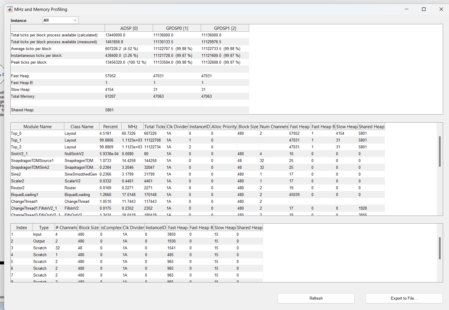
The processing takes 607k cycles (line 3). The processor clock has been reduced to 146.2 MHz and thus there are 1.462M clock cycles available (line 2). Using the traditional elapsed time method of profiling, we would report the CPU load as:

607k/1.462M = 41.5%

which is clearly wrong. The new method reports it as:

607k/13.44M = 4.52%

which is correct. When moderately loaded, we measure:

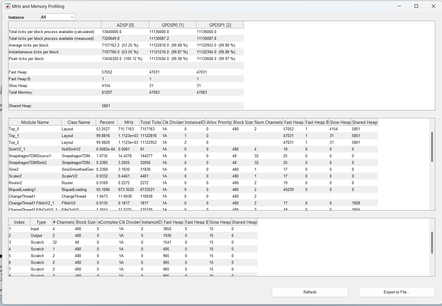
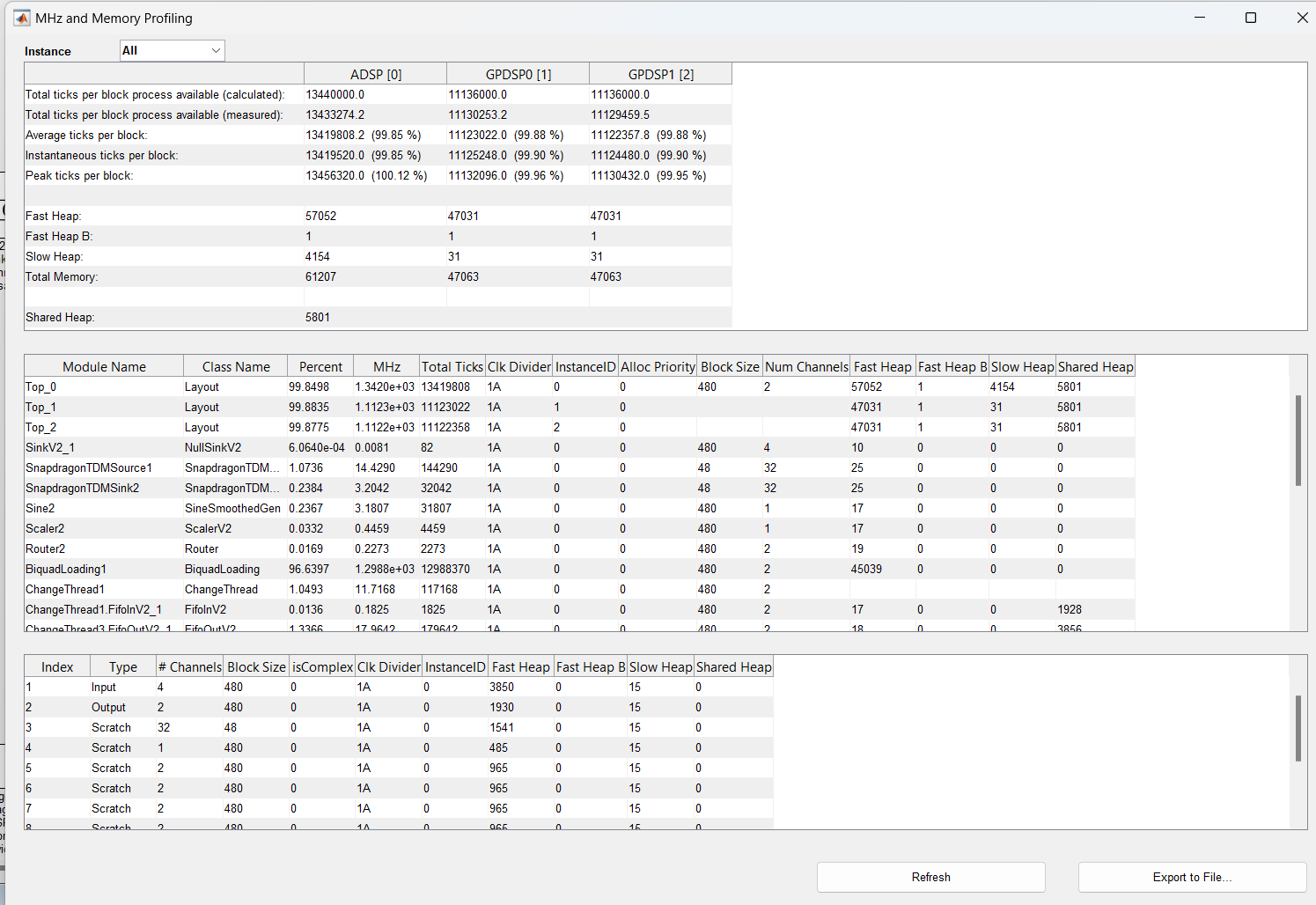
The processing requires 715.7 MHz (line 3) and the processor is running at 732MHz (line 2). We still correctly report the load as 53.25%. And finally, when the processor is heavily loaded, we now report 99.85%. In all cases, the reported load is correct even when the processor clock speed is varying.

Multirate Processing

Audio Weaver allows modules to change the block size of their output as long as they keep the block time the same as the input. Consider the system shown in Figure 23. The top path is the same as the simple system shown earlier. In the middle section, we upsample from 48 kHz to 96 kHz. The block size also doubles from 16 samples to 32 samples. The block time remains unchanged at 1/3 msec. On the bottom path, the RMS module computes the root-mean-square value of a 16 sample input block and outputs a single value. (Wires with a block size of 1 are called control wires in Audio Weaver.) The output updates every 1/3 msec which corresponds to a 3 kHz sample rate (shown on the wire). This value is filtered by SOF3 and shown on Meter1. As in the other 2 signal paths, the processing still occurs every 1/3 of a msec. Thus, this is still a single threaded system with a single layout. Hold tight; more sophisticated multithreaded processing is described in Section 3.2.

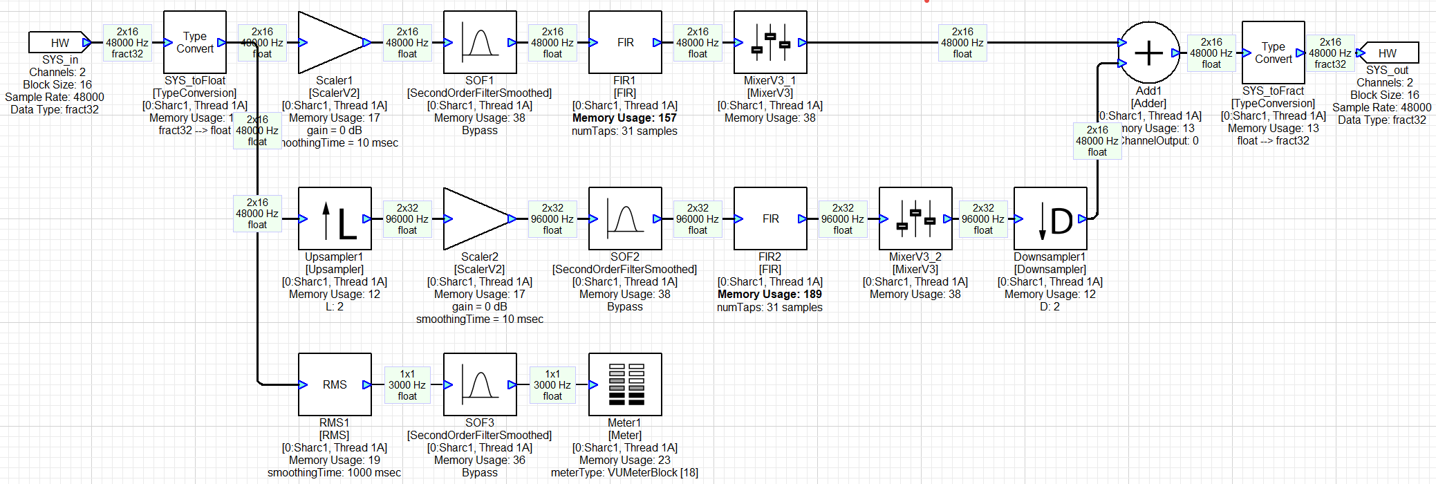
Figure . Basic multirate processing in a single threaded system.

Module Status

For simplified debugging and run-time configuration, modules in Audio Weaver have a tunable module status. The module status can be changed during design time or at run-time by right-clicking on a module as shown below.

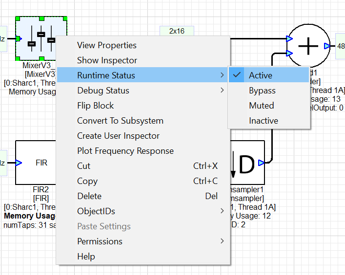
. There are 4 possible choices for the module status:

1. Active -- the module's processing function is called and is processing audio. This is the default behavior of a module when it is instantiated in Audio Weaver.

2. Bypassed -- the module's processing function is not called. Instead, the input wire data is copied to the output wire. Audio Weaver has a generic bypass function which works in the majority of cases. However, a module can define a custom bypass function, if needed (e.g., when bypassed, the Upsampler in Figure 23 continues to call its processing functions).

3. Muted -- the output wires are filled with all zeros.

4. Inactive -- nothing happens and the output wire buffer is unchanged.

When a module is Bypassed or Muted, the output wire buffers are still written and the module will consume some processing. The lowest processing occurs when the module in Inactive, but you must be careful. When Inactive, the module's output wire buffer is untouched and will contain whatever data was in there earlier. For example, consider the system shown in Figure 21. When Scaler1 is set to Inactive, it will essentially be Bypassed since the module operates in-place and Wire 1 holds Scaler1's input data. However, when SYS_toFloat is bypassed, Wire 1 holds fixed-point data. This will be treated as floating-point by Scaler1 and will result in very loud noise. Be careful when using Inactive mode and consider the possible consequences.

Multithreaded Processing

Single threaded processing is useful for basic audio designs. More sophisticated algorithms, or running multiple use cases simultaneously, require processing audio in multiple threads.

Suppose you are running road noise cancellation with a block size of 0.33 msec (16 samples at 48 kHz). In addition, you want to do playback processing on the same core. You could do the playback processing also at a 0.33 msec block size, but that would be inefficient. It would be better to do it at a larger block size, like 1.33 msec (64 samples). To achieve this requires a multithreaded implementation.

To switch from a block size of 16 samples to 64 samples requires double buffering as shown in Figure 24. There are 2 ping pong buffers with 64 samples each. Input Buffer A is filled 16 samples at a time while Input Buffer B is used for processing. After the input buffer is full (or output buffer is empty), then the buffers switch. Processing then occurs with Buffers A and I/O with Buffers B.

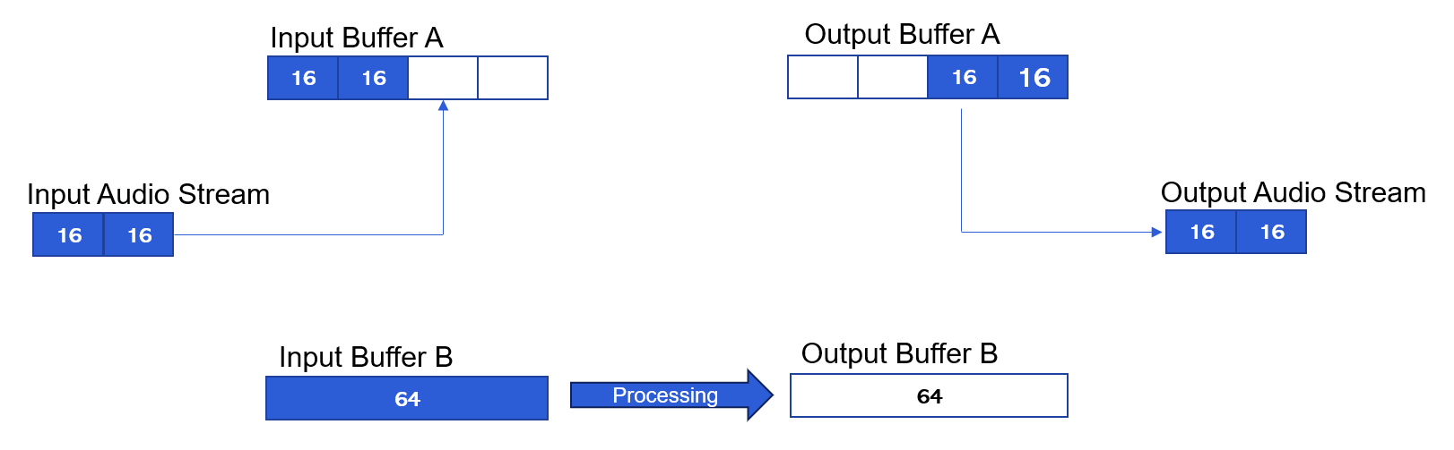
Figure . Double buffering required for multithreading. In the example, audio arrives at a block size of 16 samples and is buffered up to 64 samples.

Layouts and Clock Dividers

In Audio Weaver, the 16 and 64 sample processing occur in separate layouts. Each layout has an ordered list of modules to execute. The smallest block size in the system is triggered off the basic block size. Within this interrupt, the 16 sample processing occurs every call and every 4^th^ call we trigger a lower priority thread for the 64 sample processing. In Audio Weaver, we would state that the 64 sample layout is running at a clock divider of 4.

Processors with Hardware Threads

On a processor like the Hexagon which has hardware threads, these threads execute at the same time. The pattern of processing is as shown in Figure 25. Multithreading on the Hexagon increases the total amount of audio compute. You must use multiple threading to fully leverage the Hexagon.

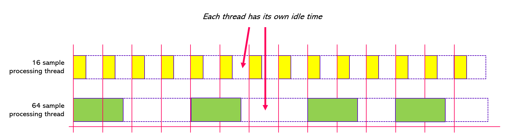
Figure . Multithreaded activity in the Hexagon processor. The 2 block sizes execute in parallel on separate hardware threads.

Processors without Hardware Threads

On a processor like the SHARC which doesn't have hardware threads, the processing occurs in separate software threads. The 16 sample processing operates in a higher priority thread and interrupts the 64 sample processing. The processor can only do 1 thing at a time and the pattern of processing is shown in Figure 26. Multithreading on the SHARC does not increase the total amount of audio compute available; it only allows you to process at different block sizes.

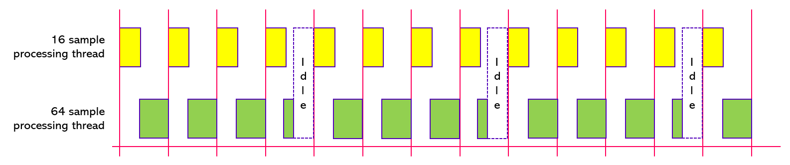
Figure . Multithreaded processing on the SHARC. It has only a single hardware thread and the high priority software thread (in yellow) interrupts and preempts the lower priority thread (in green).

The 16 and 64 sample processing are supposed to occur at the same time as shown above, but since the core can only do 1 thing at a time, the higher priority 16 sample processing occurs. Then, when the 16 sample processing is done, the 64 sample processing can begin. The 64 sample processing takes longer to execute and is repeatedly pre-empted by the higher priority thread. The processor is idle only after the 64 sample processing is done.

Measuring CPU load

Measuring the CPU load with parallel running hardware threads is simple. Just measure \(T_{B}\) and \(T_{P}\) for each thread and compute the statistics as before. You end up with a % loading for each hardware thread. With software threads, computing the loading is more difficult because the low priority thread is pre-empted by the high priority thread. Just measuring \(T_{B}\) and \(T_{P}\) for the low priority thread will include the time spent in the high priority thread. To avoid this, the Audio Weaver has additional code to ignore the time spent in higher priority threads.

Latency Due to Multithreading Buffering

When implementing multithreading, you also need to consider the latency which occurs from double buffering. A detailed analysis is shown in Figure 27. 16-sample blocks A, B, C, and D arrive. Then the 64 sample block -- ABCD -- can be processed. After this is complete, the results A, B, C, and D can be output. The analysis shows that the delay from buffering up is 64 samples and buffering down adds another 64 samples. The net latency then is 128 samples, or 2.67 msec.

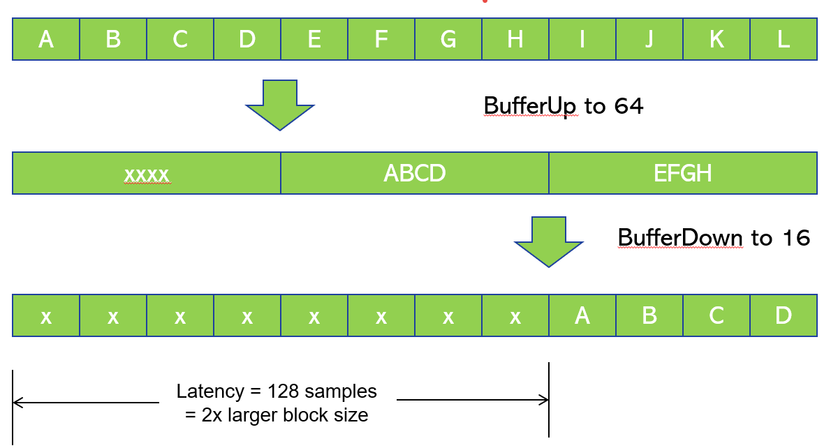
Figure . Latency that occurs from the buffering used in multithreaded systems.

Audio Weaver ChangeThread Module

Thread management is performed in Audio Weaver using the ChangeThread module. This module includes an internal double buffer (twice the larger block size) and changes the thread identifier for downstream modules. During design time, you specify the number of blocks which should be accumulated (when buffering up) or subdivided (when buffering down). The thread information (and block size, sample rate, and number of channels) propagates through the signal flow from module-to-module. An example implementation with RNC at 0.33 msec and playback processing at 1.33 msec is shown in Figure 28.

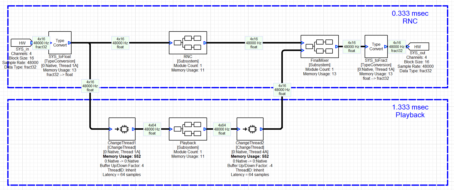
Figure . Basic multithreaded system implemented in Audio Weaver. The high priority thread is in the upper path and has a block size of 0.33 msec. In the lower path, audio is buffered up to 1.33 msec, processed by Playback, and then buffered down to 0.33 msec.

Multithreading at the same block size

The ChangeThread module also allows you to switch to another thread at the same block size. This is useful on the Hexagon (but not on the SHARC) because it increases the total available processing available. A basic 2 thread design is shown in Figure 29. The block size is 1 msec throughout the system. The first three modules execute in thread 1A while the last three modules execute in thread 1B.

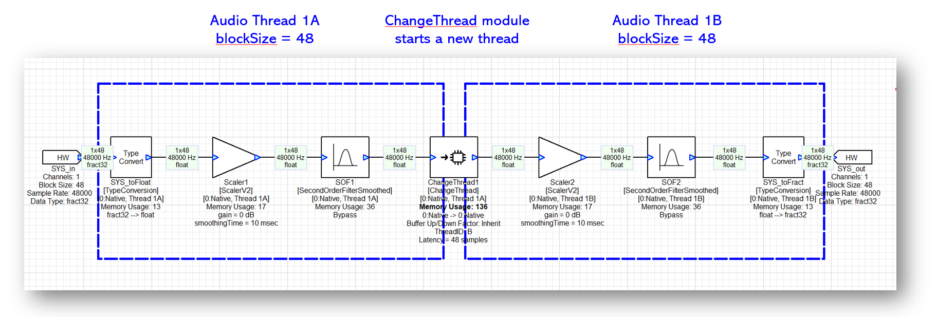
Figure . Multithreading works even if you don't change the block size.

Keep in mind that the ChangeThread module still includes double buffering in this example, and that the 2 parts of the system execute in parallel as shown in Figure 30. The ChangeThread module also add 1 block of latency (48 samples) in this example.

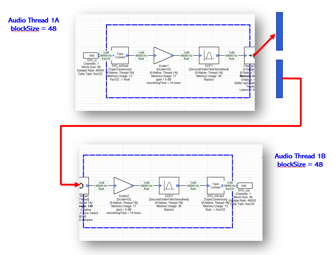
Figure . In this multithreaded design, both threads process 1 msec of audio and execute in parallel.

awe_audioGetPumpMask()

This API is called by the main DMA handler (at the smallest block size) and returns a bit mask which indicates which audio thread(s) are ready to run. The signature for the function is

INT32 awe_audioGetPumpMask(AWEInstance* pAWE);

The least significant bit of the return value corresponds to the highest priority audio processing thread in the system.

For example, suppose that the system has a basic block size of 1 msec. Furthermore, assume that the system processes audio with block sizes of 1 msec, 2 msec, and 5 msec. The bit mask returned by the function will have the following values (shown in binary) during each 1 msec interrupt

111 // Call 0

001 // Call 1

011 // Call 2

001 // Call 3

011 // Call 4

101 // Call 5

011 // Call 6

001 // Call 7

011 // Call 8

001 // Call 9

111 // Call 10

The least significant bit is set every time so that the 1 msec audio thread is triggered every time.

Multicore Processing

Audio Weaver also allows you to partition processing across multiple cores. The approach used is an extension of the multithreaded architecture described in the previous section. The design places relatively few requirements on the underlying hardware. We assume:

(1) Each processor has its own local tightly coupled memory which cannot be accessed by the other cores. This tightly coupled memory is used for speed intensive operations.

(2) The cores all have access to a common pool of shared memory.

(3) The cores are able to signal each other via interrupts.

(4) One or more of the cores have access to hardware peripherals for I/O.

This architecture even supports heterogeneous configurations of cores and is illustrated in Figure 31.

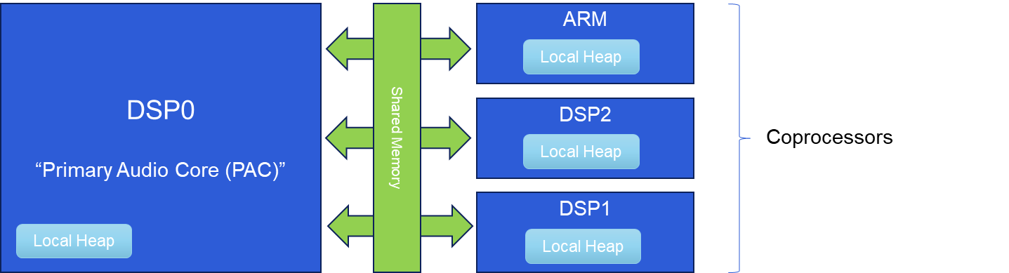
Figure . Internal SOC architecture needed to support heterogeneous multicore processing.

DSP0 is the "Primary Audio Core (PAC)" and performs I/O at the basic block size. The other "Coprocessors" process audio at multiples of the basic block size. The Coprocessors are signaled by the PAC based on their clock dividers. The PAC is essentially the conductor which keeps the entire cluster of processors synchronized.

The cores communicate via double buffers as before in the multithreaded design. The only difference is that the double buffers are allocated in shared memory. While one buffer is being filled, the other is being used for processing.

The ChangeThread module which was introduced earlier also allows you to specify the target core ID of subsequent processing. The target core ID is then propagated to downstream modules just as the threadID was propagated earlier. A useful feature of the ChangeThread module is that you can change the block size (buffering up or buffering down) at the same time as crossing to another core. Figure 32 shows an example of how the ChangeThread module is used. Core 0 is the interrupt controller and implements low latency RNC and a final mixer / limiter at a block size of 0.5 msec. Core 1 performs playback processing with a block size of 5 msec while Core 2 does voice processing with a block size of 10 msec.

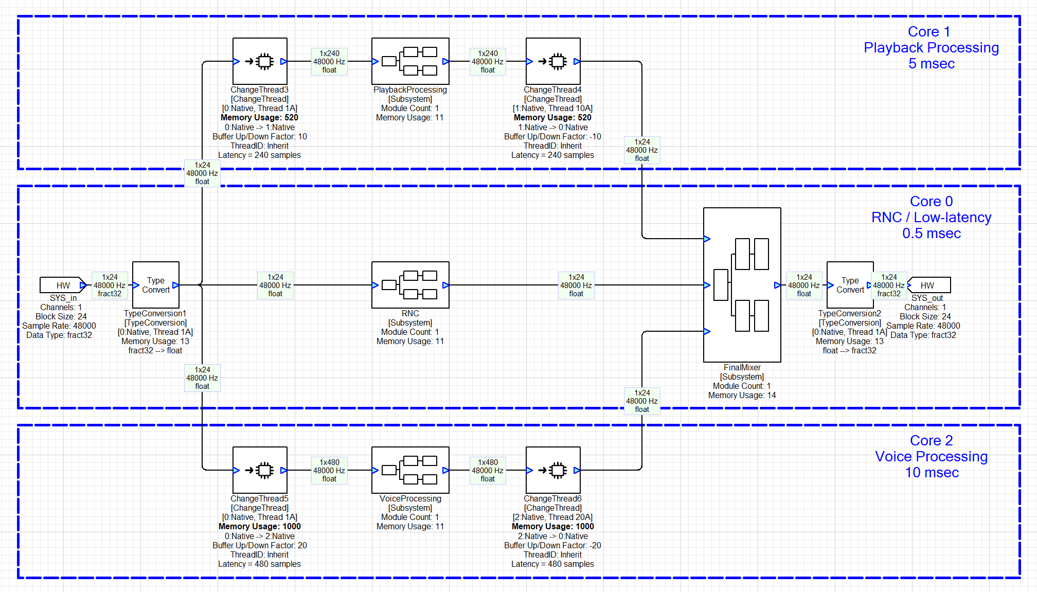
Figure . Extension of Audio Weaver processing to multiple cores. The ChangeThread module is able to simultaneously span core boundaries and change block sizes.

Synchronous Operation

Audio Weaver's real-time architecture is based on fully synchronous operation. Audio processing occurs in fixed block sizes, and block sizes through the system are multiples of the basic block size of the system. This provides consistent CPU loading (no spikes), fixed scheduling, and efficient use of computational resources.

The PAC manages DMA at the basic block size of the system. After every buffer is received, the PAC calls the function

INT32 awe_audioIsReadyToPumpMulti(AWEInstance* pAWE, UINT32 instanceID);

where the second argument instanceID is the core ID of the Coprocessor. This function returns a Boolean which indicates whether a thread on the Coprocessor is ready to pump. If true, then the PAC will signal the Coprocessor to process audio.

Audio Weaver's multicore architecture allows you to leverage additional threads within each core. In the 3 core design shown in Figure 32, suppose that each core contained the following block sizes / clock dividers:

• Core 0: 0.5 msec, 0.5 msec, 4 msec, 20 msec

• Core 1: 5 msec, 5 msec, 5 msec, 5 msec

• Core 2: 10 msec, 10 msec, 20 msec, 20 msec [Core 2 wakes up every 10 msec based on IPCC]

• Core 3: 4 msec, 10 msec. [GCD = 2 msec. Core 3 wakes up every 2 msec.]

• Core 4: 10 msec, 11 msec. [GCD = 1 msec. Core 4 wakes up every 1 msec.]

Processing is fully synchronous and triggered by the 0.5 msec interrupt controller. The system wide pattern of audio processing ("pumping") is shown in Figure 33.

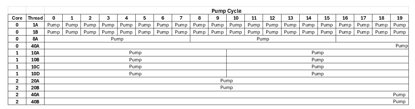
Figure . System with 3 cores and each core implements 4 threads at different block sizes.

This architecture imposes some restrictions as to how block sizes can be used. Here are some examples:

• An algorithm cannot change its block size on the fly at run-time. (To realize this, you'll need to operate the two algorithms in parallel and Active / Inactivate the processing at run-time. You'll need twice the memory, but the CPU load is constrained.)

• Algorithms with block sizes of 240 and 256 samples cannot be directly cascaded. (To accomplish this, you would need a basic block size of 16 samples. You would have to first buffer down from 240 to 16 samples and then buffer up from 16 to 256 samples. This places the modules into layouts with clock dividers to 15 and 16.)

• Asynchronous sample rate conversion cannot be supported (easily) in the design since wires have fixed block sizes.

Resynchronization

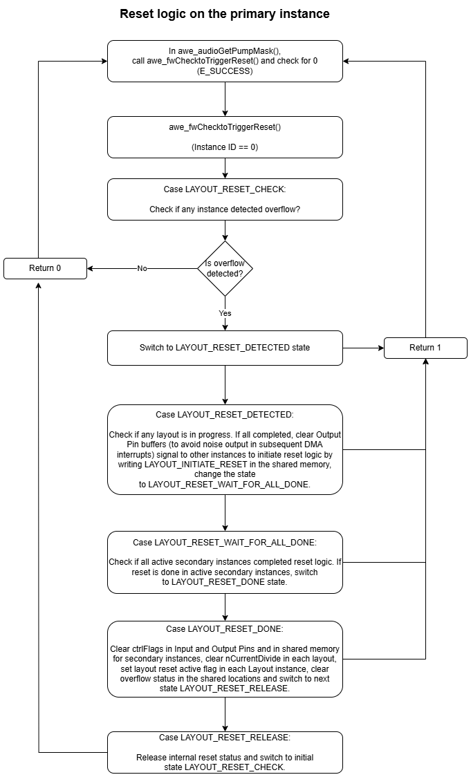
The AWECore processing library has internal logic which checks for CPU overruns (not completing processing in time for the next interrupt), and when detected, it pauses pumping and resynchronizes all threads.

Part of the resynchronization logic is in the function awe_audioGetPumpMask(). In the logic that computes the pump mask, we check to make sure that any thread to be started has finished its previous pump cycle. If it hasn't, then we set a "PUMP_OVERFLOW" bit in the layout structure and do not set the corresponding bit in the layout mask (that is, don't start this thread again). When an overflow occurs in a layout on some core, then we share this information with the PAC by setting an overrun bit set in a dedicated location in the shared heap for that core.

Another possible overrun is with FiFoIn and FiFoOut in ChangeThread module. In multi-core system, FiFoIn runs on one core and FiFoOut runs on a different core. In normal operation, they both remain synchronized, i.e. FiFoIn writes into first half while FiFoOut reads from the second half of the double buffer in shared heap. If either FiFoIn or FiFoOut is delayed due to other system events, this is detected as an overrun and a flag in the dedicated shared heap header set to indicate overrun.

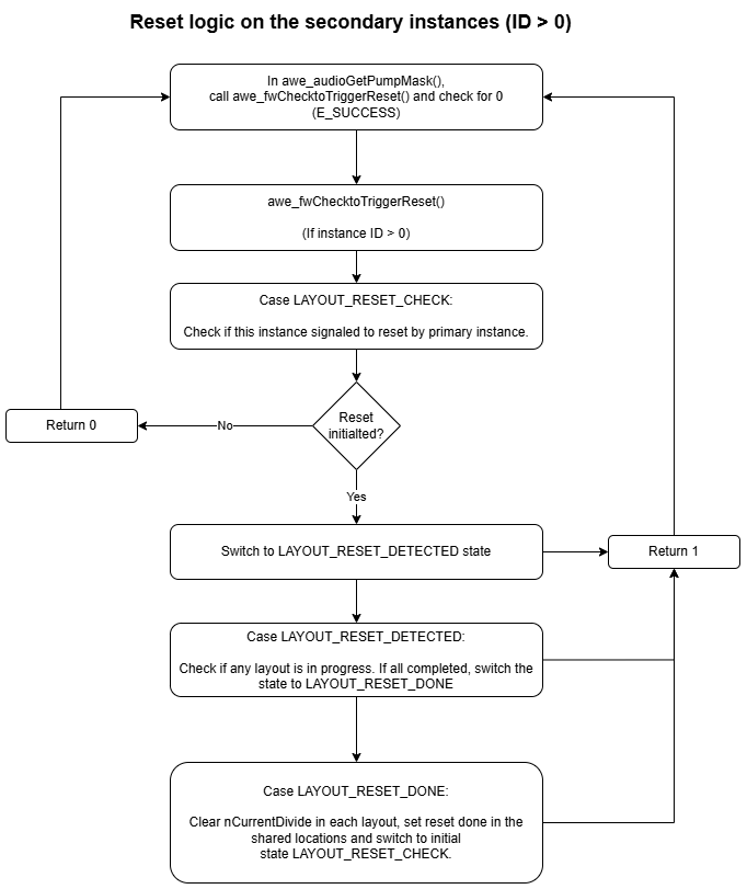
The awe_audioGetPumpMask() function on the PAC (instance 0) keeps checking the shared heap for any overruns occurring on any core. If an overrun detected anywhere in the system, the resynchronization state machine starts and acts for every call to awe_audioGetPumpMask. First instance 0 signals all other instances to start resynchronization. Then all instances wait until all the current pumps to complete. Depending on the load of each instance, it may take a variable number of fundamental blocks to complete this state. Then in the next fundamental block period, instance 0 resets hardware I/O pin double buffer flags and resets all the layout flags. Then instance 0 waits for all other instances to complete reset. After one block of fundamental block period, after all instances completed resynchronization, then the normal execution takes place. The following flow diagram provides more details on state machine in the PAC and Coprocessor instances

.

Deferred Processing

Audio Weaver contains a separate Deferred Processing Thread for handling non-real-time module operations. The Deferred Processing Threads runs at a priority lower than any of the real-time audio processing threads. This ensures that control and tuning operations do not interfere with real-time audio.

Module Architecture

This section describes the architecture of individual modules that can be used by Audio Weaver. It provides a high-level understanding of the design and capabilities of modules. More detailed information aimed at module developers is found in the Audio-Weaver--Module-Developers-Guide.

Code and data for a module can be roughly divided into two categories. Information which resides on the PC and enables the module to be used in Designer. This includes graphical information, variable details, GUI inspector, and so forth. This information is contained in either MATLAB code or separate files. The second part of a module is code which runs on the target processor (or inside the Native PC simulator). The components are:

On the PC

• ClassName_module.m -- MATLAB code which describes the pins, variables, and Designer behavior of the module. A class-based approach is used with multiple internal methods. This is the source of truth.

• ClassName.xml -- XML code which is read by Designer. This is used to populate the Module Browser found on the left-hand side of the Designer GUI. This is auto-generated based on the _module.m file.

• ClassName.bmp -- bitmap file used in the Module Browser.

• ClassName.svg -- Vector graphics file used to draw the module on the Designer canvas.

• ClassName.html -- Help documentation.

On the target

• ModClassName.c -- C code with multiple internal functions:

  • Constructor() -- for memory allocation

  • Process() -- real-time processing

  • Set() / Get() -- for run-time control

  • Bypass() -- defines the module's bypass functionality

• ModClassName.h -- Header file with module structure definitions

On the PC, your custom modules will be contained in DLL's which are loaded by the Server upon startup[^5]. The DLL contains the run-time code (from ModClassName.c) and also "schema" information which is a text-based description of the module's instance variables.

Arguments and Variables

Arguments in Audio Weaver are module configuration settings which affect memory allocation and wiring. Arguments can only be set at design time and not when the system is running. Examples are:

• Length of an FIR filter.

• Number of stages in a Biquad filter.

• Decimation factor of the Downsampler module.

• Number of input pins on an Interleaver module.

Variables exist on the target and are available to the Process() and Set() functions. Variables can be further classified based on how they are used:

Parameters -- set by the user (e.g., the frequency, gain, and Q of a peaking filter).

Derived -- internal variables which are computed by a module's Set() function (e.g., Biquad coefficients computed based on frequency, gain, and Q of a peaking filter).

State -- internal variables which are modified by a module's Process() function (e.g., the 2 state variables used by a direct form 2 Biquad filter).

Arguments exist primarily in the MATLAB but may be assigned to variables when needed by the run-time code.

Module Instance Structure

Each module has an associated instance structure which holds its variables. The instance structure consists of a common header used by all modules, followed by module specific variables. Here are some examples:

Abs -- computes the absolute value of a signal. No tunable parameters.

typedef struct _awe_modAbsInstance
{
    ModuleInstanceDescriptor instance;
} awe_modAbsInstance;

ScalerDB -- Scaler with configurable gain in dB. No smoothing[^6].

typedef struct _awe_modScalerDBInstance
{
    ModuleInstanceDescriptor instance;
    FLOAT32 gainDB; // Gain in dB.
    FLOAT32 gain; // Gain in linear units.
} awe_modScalerDBInstance;

ScalerNV2 -- N channel scaler with per channel gain settings. Smoothed.

typedef struct _awe_modScalerNV2Instance
{
    ModuleInstanceDescriptor instance;
    FLOAT32 masterGain; // Overall gain to apply.
    FLOAT32 smoothingTime; // Smoothing time constant (msec).
    INT32 isDB; // Selects between linear(=0) and dB(=1)
    FLOAT32 smoothingCoeff;// Smoothing coefficient.
    FLOAT32* trimGain; // Array of trim gains, one per channel
    FLOAT32* targetGain; // Computed target gains in linear units
    FLOAT32* currentGain; // Instantaneous gains.
} awe_modScalerNV2Instance;

Every module starts with the common header:

ModuleInstanceDescriptor instance;

This is the base class of the module and contains information common to all modules (access to wires, module status, etc.). Note that the instance structures don't contain information about number of wires, block sizes, number of channels, or sample rate. This information is encoded into the wire buffers and queried by the module functions. You can see this in the Process() function for the ScalerDB module shown below:

void awe_modScalerDBProcess(void *pInstance)
{
    awe_modScalerDBInstance *S = (awe_modScalerDBInstance *)pInstance;
    **WireInstance **pWires = ClassModule_GetWires(S);**
    UINT32 channels, blockSize;
    **UINT32 numPins = ClassModule_GetNInWires(S);**
    UINT32 pin;
    FLOAT32 *src,*dst;
    for(pin=0;pin<numPins;pin++)
    {
        src = (FLOAT32 *)(pWires[pin]->buffer);
        dst = (FLOAT32 *)(pWires[numPins+pin]->buffer);
        **channels = ClassWire_GetChannelCount(pWires[pin]);**
        **blockSize = ClassWire_GetBlockSize(pWires[pin]);**
        /* The same gain is used for all channels */
        awe_vecScale(src, 1, dst, 1, S->gain, blockSize*channels);
    }
}

Figure . Process() function for the ScalerDB module. The highlighted lines show how common module information (number of pins, channels, and block size) can be queried via macros.

Module C Functions

Modules have several C functions which control their behavior. Every module needs a Process() function while the others are optional.

Constructor()

This is an optional function and usually is needed if the module requires additional memory allocation or extra initialization. If a module only contains scalar variables in the instance structure (like the ScalerDB module above), then a Constructor() is not required. The ScalerNV2 module shown above has several array variables whose size is based on the number of channels. Here is its Constructor():

ModInstanceDescriptor *awe_modScalerNV2Constructor(INT32 * FW_RESTRICT retVal, UINT32 nIO, WireInstance ** FW_RESTRICT pWires, size_t argCount, const Sample * FW_RESTRICT args)
{   
    awe_modScalerNV2Instance *S = (awe_modScalerNV2Instance *) BaseClassModule_Constructor((ModClassModule *) &awe_modScalerNV2Class, retVal, nIO, pWires, argCount, args);

    // Check if BaseClassModule_Constructor() finished properly.  If not,
    // the error code is in *retVal
    if (S == NULL)
    {
        return 0;
    }

    #if defined(AWE_PROCESSOR_LOCK)
    {
        UINT32 nID = S->instance.instanceDescriptor.nUniqueInstanceID;
        *retVal = nID;
        awe_fwSetPackedVersion(retVal);
        if (*retVal == nID)
        {
            *retVal = E_SUCCESS;
        }
        else
        {
            *retVal = E_CRC_ERROR;
            return 0;
        }
    }
    #endif

    if ((S->trimGain = (FLOAT32 *) awe_fwMalloc(ClassWire_GetChannelCount(pWires[0]) * sizeof(float), AWE_HEAP_FAST2SLOW, retVal)) == 0)            
    {            
        // Error code is in *retVal            
        return 0;            
    }            

    if ((S->targetGain = (FLOAT32 *) awe_fwMalloc(ClassWire_GetChannelCount(pWires[0]) * sizeof(float), AWE_HEAP_FAST2SLOW, retVal)) == 0)            
    {            
        // Error code is in *retVal            
        return 0;            
    }            

    if ((S->currentGain = (FLOAT32 *) awe_fwMalloc(ClassWire_GetChannelCount(pWires[0]) * sizeof(float), AWE_HEAP_FAST2SLOW, retVal)) == 0)            
    {            
        // Error code is in *retVal            
        return 0;            
    }            


    return ((ModInstanceDescriptor *) S);            


}

The call to BaseClassModule_Constructor() allocates memory for the module instance structure, assigns all scalar variables, and assigns wire information. This is then followed by 3 calls to awe_fwMalloc() to allocate memory for the gain arrays. The number of channels is determined by the macro ClassWire_GetChannelCount() and memory is allocated from the Audio Weaver heaps. More information about Audio Weaver heaps can be found in Section 4.4.

After the Constructor is complete, memory has been allocated for the array variables, but they have not yet been initialized to their default values.

Process()

Required function for every module. This implements the processing, and the code for the ScalerDB module was shown earlier in Figure 34. For greatest flexibility, you should write modules so that they can support an arbitrary block size and number of channels. A module's wire restrictions are specified in MATLAB code and MATLAB enforces that these conditions at build time. Your module's C code does not have to do additional checking of the wire properties.

The module processing function is usually written in C code. If you need additional performance, you can call hand optimized functions written in assembly. DSP Concepts' library of optimized functions is called the Vector Library. It contains a wide variety of low-level primitives like Biquad filters, Scalers, Smoothed Scalers, FIR filters, and so forth, that have been optimized for many different processor architectures.

Some processors include specialized hardware to accelerate specific functions like ML inference, FFT, IIR, and matrix accelerators. You can call these processor-specific APIs from your module code. Audio Weaver's SHARC library leverages some accelerators.

Bypass()

This is an optional function if a module needs special behavior when it is bypassed. The function header is exactly the same as the Process() function. For example, when bypassed, the TypeConvert module continues to call its Process() function. Not doing so would lead to serious distortion.

Set()

Used for run-time control and allows you to convert tunable parameters to derived variables. The ScalerDB module demonstrates how this works. The tunable variable gainDB needs to be applied as a linear gain. Instead of converting in the module's Process() function (this is wasteful of CPU), it is better to define a Set() function as shown below:

UINT32 awe_modScalerDBSet(void *pInstance, UINT32 mask)
{
    awe_modScalerDBInstance *S;

    S = (awe_modScalerDBInstance *)pInstance;
    S->gain = undb20f(S->gainDB);

    return 0;
}

The Set() function has two input arguments. The first is a pointer to the module's instance structure. The second is a mask which indicates which variable(s) in the module have been changed. This allows you to do selective computation in the Set() function. The constant MASK_ScalerDB_gainDB is defined in the module's header file (ModScalerDB.h).

The Audio Weaver framework is designed to directly set variables in module structures during run-time control or tuning. When controlling the ScalerDB module, the framework would first write gainDB and thereafter call the Set() function. We go into more detail into the Audio Weaver control architecture in Section 5.

The module's Set() function is called automatically after its Constructor() with mask = 0xFFFFFFFF. This is used to compute default derived values at startup. The Set() function is also called with mask=0 when the system is being destroyed. This can be used by the module if it needs to cleanup before shutting down (e.g., close a file or deallocate memory that was allocated outside of the Audio Weaver heaps).

Get()

This module function is rarely used by has complementary behavior to the module's Set() function. The Get() function is used to do a specific calculation before reading back an instance variable. For example, the SoftClip module applies a point nonlinearity to a signal. If you want to know the specific gain which is applied (the currentGain variable in the instance structure), then you need to perform a division. Instead of burdening the Process() function with this math, you can define a Get() function as shown below:

UINT32 awe_modSoftClipGet(void *pInstance, UINT32 mask)
{
    awe_modSoftClipInstance *S = (awe_modSoftClipInstance *)pInstance;
    WireInstance **pWires = ClassModule_GetWires(S);
    INT32 numChannels = ClassWire_GetChannelCount(pWires[0]);
    INT32 ch;

    for (ch = 0; ch < numChannels; ch++)
    {
        if (S->lastIn[ch] != 0.0f)
        {
            S->currentGain[ch] = S->lastOut[ch] / S->lastIn[ch];
        }
    }

    return 0;
}

Memory Allocation

Audio Weaver manages 4 internal memory heaps that can be used by modules. This design is specifically for DSP processors which have different internal and external memory blocks. The heaps are called: FAST, FASTB, SLOW, and SHARED. FAST and FASTB are typically in internal memory and support the dual access required to efficiently implement FIR filters. FAST would hold the filter coefficients and FASTB would hold the state variables. SLOW is usually much larger and mapped to external memory. Finally, SHARED memory is a recent addition and is available only in SOCs that support shared memory. The SHARED heap is used to implement interprocessor communication via the Change Thread module.

FAST, FASTB, and SLOW are local to each audio processor core. Only the SHARED memory is visible to everyone. Often FAST and FASTB are placed in TCM for better performance.

Audio Weaver also supports a single heap design which combines FAST, FASTB, and SLOW. This is for processors which have a unified flat memory space, like an Arm Cortex-A[^7].

Memory allocation from the Audio Weaver heaps is via the function

void *awe_fwMalloc(UINT32 size, UINT32 heapIndex, INT32 *retVal);

You specify the SIZE in bytes and which heap to allocate from via heapIndex. The function returns a pointer to the allocated memory as a void * or upon failure returns an error code in retVal. There is a lot of flexibility in the heapIndex. You can specify a single heap, AWE_HEAP_FAST, or a hierarchy of heaps like AWE_HEAP_FAST2SLOW. This first tries to allocate in FAST. If this is full, then it tries FASTB. And finally, if this is full, it attempts to allocate in SLOW.

The AWECore library can be configured at initialization to perform aligned memory allocations. This ensures that all wires buffers and array variables are aligned. Here are typical settings:

Processor Alignment (bytes)

---

X86 16 Arm Cortex-A 16 SHARC+ 16 SHARC FX 4 Arm Cortex-M 4 HiFi 4 16 HiFI 5 16 Hexagon 16 CEVA-X2 16 TI C6x 16 TI C7x 32

The alignment settings may change from build-to-build. The alignment settings of the currently connected target are shown on the Server. See Figure 7.

Audio Weaver does not support freeing individual blocks of memory. We avoid this because it leads to memory fragmentation and is not a good choice for deeply embedded systems. When a system is destroyed, Audio Weaver frees all heap memory and sets the contents to zero in preparation for the next design. You never have to free() memory allocated from the Audio Weaver heaps.

Modules are permitted to do memory allocation themselves outside of the Audio Weaver heaps. This often occurs in you are using C++ code or if you are wrapping an IP library that does its own allocation. Note that this "hidden" memory won't be visible to Audio Weaver and won't be captured by its profiling features. Also keep in mind that you have to manually free() memory when the system is destroyed. This is usually handled in your module's Set() function when MASK == 0. See Section 4.5.6.7.

Module MATLAB Functions

Every module in Audio Weaver has associated MATLAB code which describes the module's capabilities and variables. This is implemented in Audio Weaver as an @awe_module class object. This section follows the ScalerDB module and shows relevant parts of the code. The ScalerDB module is contained in the file scaler_db_module.m.

scaler_db_module.m Walk Through

The entry point of this function is referred to as the MATLAB Constructor. It creates and returns an @awe_module object which contains the ScalerDB module. The top of the function contains the standard MATLAB function header:

function M=scaler_db_module(NAME,NUMPINS)
% M=scaler_db_module(NAME, NUMPINS) 
% Creates a dB scaler for use with the Audio
% Weaver environment. The scaler has a single multichannel input and scales
% all channels by the same value. 
% 
% Arguments:
%    NAME - name of the module.
%    NUMPINS - Optional: number of inputs. Default = 1 input, 1 output.
%       The ith input pin is then scaled and placed in the ith output
%       pin. In all cases, the same scale factor is applied to all values.


% Copyright 2007.  DSP Concepts, Inc.  All Rights Reserved. 
% Author:  Paul Beckmann

% AudioWeaverModule [This tag makes it appear under awe_help]

% ----------------------------------------------------------------------
% Create the low-level object with render variables
% ----------------------------------------------------------------------

if (nargin < 2) || isempty(NUMPINS)
    NUMPINS=1;
end

if NUMPINS < 1
    error('ScalerDB module requires at least 1 input pin!');
end

The first argument to every Audio Weaver module function is the NAME of the module in the system. Then there is an optional argument (same as arguments from Section 4.1) which indicates how many input pins the module should have. The module then sets default arguments for NUMPINS and checks that it is a positive integer.

The next part of the code creates the @awe_module object and adds arguments.

M=awe_module('ScalerDB', 'Gain control with dB units and no smoothing');
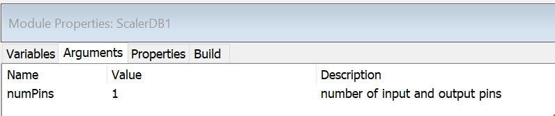
add_argument(M, 'numPins','int', NUMPINS, 'const', 'number of input and output pins');


if (nargin == 0)
    return;
end

The function returns if (nargin == 0) which means that no arguments, not even the NAME, was supplied to the function. This is provided so that Designer can easily query how many arguments a module takes without going through the entire instantiation process. With this code, Designer is able to present numPins as an argument that the user can edit:

The string 'ScalerDB' is the class name of the module and plays a vitally important role. This must be unique within the Audio Weaver module class name space. We recommend that you use your company name to generate unique names, like 'MyCompanyScalerDB'. The class name must be a valid C variable name and will be used to generate a variety of file names and variable names.

Next the name of the module is set based on the first argument NAME. The module also provides a defaultName which is used to generate the name when the module is dragged out in Designer. The defaultName is 'ScalerDB' and the first instance will be named "ScalerDB1", the second instance "ScalerDB2", and so forth.

M.name=NAME;
M.defaultName = 'ScalerDB';
M.processFunc=@scaler_db_process;
M.freqRespFunc=@scaler_db_freq_response;
M.testHarnessFunc = @test_scaler_db;

The module is then marked as deprecated. That means that there are newer modules which perform the same function. (Deprecated modules can continue to be used but are drawn in grey on the Designer canvas.)

M.isDeprecated = 1;

Input and output pins are then added to the module. NUMPINS inputs and NUMPINS outputs are added.

PT=new_pin_type([], [], [], 'float', []);


add_pin(M, 'input', 'in', 'Input signal', PT, NUMPINS);
add_pin(M, 'output','out', 'Output signal', PT, NUMPINS);

The new_pin_type.m function returns a structure, PT, which describes the properties of the pin. It specifies what wire properties the module can support. The arguments to this function are:

PT = new_pin_type(NUMCHANNELS, BLOCKSIZE, SAMPLERATE, DATATYPE, ISCOMPLEX);

NUMCHANNELS, BLOCKSIZE, and SAMPLERATE specify the properties of wires that can be connected to the pin. Audio Weaver Designer automatically validates connections when the system is built. All three properties use the same format. For example, the NUMCHANNELS you can express the following:

[] -- the empty matrix indicates that there are no constraints placed on the number of channels.

[N] -- a single value indicates that this module only supports N channels.

[M N] -- indicates that the module supports M to N channels. (Note, this is a row vector.)

[A; B; C; D] -- indicates that the module supports A, B, C, or D channels. (Note, this is a column vector.)

[M N STEP] -- indicates that the module supports, M, M+STEP, M+2*STEP, ..., N channels.

There is even more flexibility in the range constraints and this is fully described in the Audio Weaver Module Developers Guide.

DATATYPE is a string with one of these values:

'fract32' -- 32-bit fractional representation. Numbers in the range [-1 +1).

'int' -- signed 32-bit integers. Numbers in the range [-(2^31) (2^31)-1].

'float' -- single precision floating-point.

'*32' -- can be any 32-bit data type.

ISCOMPLEX indicates whether the module can support complex data.

0 = real data (the default)

1 = complex data

[] = real or complex

The ScalerDB module sets:

PT = new_pin_type([], [], [], 'float', []);

Thus, this module supports any number of channels, any block size, any sample rate, floating-point data only, and real data or complex data.

Next in scaler_db_module.m, two variables are added.

% ----------------------------------------------------------------------
% Add the target-specific state variables
% ----------------------------------------------------------------------

%Interface variable: Gain in DB
add_variable(M, 'gainDB', 'float', 0, 'parameter', 'Gain in dB.');
M.gainDB.range=[-100 100];
M.gainDB.units='dB';

%Hidden State Variable: Linear equivalent of gainDB
add_variable(M, 'gain', 'float', 1, 'derived', 'Gain in linear units.', 1);
M.gain.units='linear';

"gainDB" is a floating-point variable. The default value is 0. It is a parameter which can be set by the user. There is also a short description ("Gain in dB") which will be used throughout the generated code and documentation. Lastly, the units for this variable are set to 'dB'. This string is used to annotate inspectors.

This is then repeated for the "gain" variable. The main difference is that the module is marked as hidden and won't be visible to the user.

Each variable added to the MATLAB code is automatically inserted in the module instance structure. Recall that ModScalerDB.h contains:

typedef struct _awe_modScalerDBInstance
{
    ModuleInstanceDescriptor instance;
    FLOAT32 gainDB; // Gain in dB.
    FLOAT32 gain; // Gain in linear units.
} awe_modScalerDBInstance

The next part of the MATLAB function specifies where to find the C code for the module's Process() and Set() functions. In Audio Weaver, you specify code fragments and then ModScalerDB.c and ModScalerDB.h are automatically generated.

awe_addcodemarker(M, 'processFunction', 'Insert:InnerScalerDB_Process.c');
awe_addcodemarker(M, 'setFunction', 'Insert:InnerScalerDB_Set.c');

This code was shown earlier in Figure 34 and Section 4.3.4.

The next part of the MATLAB code indicates that the module can perform in-place processing. That is, the same wire buffer can be used for the input and output of the module.

M.wireAllocation = 'across';

If the module cannot support in-place processing, then this should be set to 'distinct' (the default).

Commands are then added which define the module's inspector.

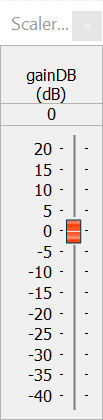
M.gainDB.guiInfo.controlType = 'slider';
M.gainDB.range = [-40 20 0.1];
add_control(M, 'gainDB');

The variable "gainDB" is exposed on the inspector. The range of the slider is -40 to +20 with a step size of 0.1. The inspector for this module is shown below.

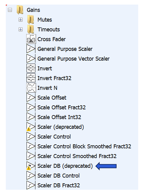
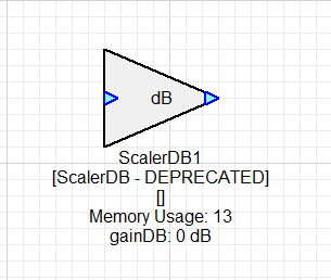
The final lines of code specify where the module appears in the Module Browser and how it is drawn on the canvas. A 32x32 pixel custom bitmap is supplied for the Module Browser and a "triangle" shape with "dB" as a legend is used for the canvas. It is also possible to specify a custom SVG file.

M.moduleBrowser.path = 'Gains';
M.moduleBrowser.image = '../images/ScalerDB.bmp';
M.moduleBrowser.searchTags = 'Scaler Volume Multiply';
M.shapeInfo.basicShape = 'triangle';
M.shapeInfo.legend = 'dB';

ScalerDB MATLAB Set Function

The function scaler_db_set.m implements the MATLAB version of the module's set function. It is not absolutely required, but is used by DSP Concepts' regression test framework. This function translates the dB gain to its linear equivalence:

function M = scaler_db_set(M)
    M.gain = undb20(M.gainDB);
return;

This set function is called when the module is instantiated or if the gainDB variable is changed while in Design mode.

ScalerDB MATLAB Processing Function

This is also an optional function and it implements the MATLAB version of the module's process function. It is used by DSP Concepts' regression test framework.

function [M, WIRE_OUT]=scaler_db_process(M, WIRE_IN)

WIRE_OUT=cell(size(WIRE_IN));

for i=1:length(WIRE_OUT)
    WIRE_OUT{i}=WIRE_IN{i}*M.gain;
end

return;

Commonly Used MATLAB Functions

The 3 most commonly used MATLAB module functions -- Constructor, Set, and PreBuild, are described in this section. Less frequently used functions are described in Section 4.5.5.

Constructor

There is no specific constructor, but we refer to the _module.m function as the "constructor" since it returns the module instance object. Required.

setFunc

Computes derived variables based on tunable parameters. Optional.

preBuildFunc

Used by a module to dynamically modify the output wire properties when the system is built. If the wires are unchanged (like the scaler_db_module.m), then this function is not needed since the base class propagates wire information unchanged by default. Examples of when you need to define a preBuildFunc:

Downsampler -- the output block size and sample rate are changed.

function M = downsampler_prebuild_func(M)

blockSize = M.inputPin{1}.type.blockSize;

if (rem(blockSize, M.D) ~= 0)
    error('The downsample factor D does not evenly divide the blockSize');
else
    newBlockSize = blockSize/M.D;
end

M.outputPin{1}.type.sampleRate=M.inputPin{1}.type.sampleRate/M.D;
M.outputPin{1}.type.numChannels=M.inputPin{1}.type.numChannels;
M.outputPin{1}.type.dataType=M.inputPin{1}.type.dataType;
M.outputPin{1}.type.blockSize=newBlockSize;

return;

TypeConvert -- the output data type is changed and an internal variable is set based on the input data type.

function [M, WIRE_OUT] = type_conversion_prebuild(M)

% Detect the input dataType
switch(M.inputPin{1}.type.dataType)
    case 'float'
        M.inputType = 0;
    case 'fract32'
        M.inputType = 1;
    case 'int'
        M.inputType = 2;
    case 'fract16'
        M.inputType = 3;
    otherwise
        error('Unsupported input dataType');
end

switch(M.outputType)
    case 0
        outputTypeStr = 'float';
    case 1
        outputTypeStr = 'fract32';
    case 2
        outputTypeStr = 'int';
    case 3
        outputTypeStr = 'fract16';
    otherwise
        error('Unknown outputType');
end

M.outputPin{1}.type = M.inputPin{1}.type;
M.outputPin{1}.type.dataType=outputTypeStr;
M.outputPin{1}.type.dataTypeRange={outputTypeStr};

return;

You also need to define a preBuildFunc if the sizes of module variables change based on the wire information. An example is the Biquad filter where the preBuildFunc sets the size of the state variable based on the number of channels.

function M=biquad_prebuild_func(M)

% Set the size of the state variables based on the number of channels.
M.state.size=[2 M.inputPin{1}.type.numChannels];
M.state=zeros(2, M.inputPin{1}.type.numChannels);

M.outputPin{1}.type=M.inputPin{1}.type;

return;

Less Frequently Used MATLAB Functions

The @awe_module class has many methods that can be defined. Many of these are only used in rare cases when a module has non-standard requirements.

postBuildFunc

Rarely used. This is called if the module has to perform a specific function after all modules have been created during the build process. For example, the param_set_module.m uses this to locate the controlled module.

propagateChannelNamesFunc

Propagates custom channel name information. The base class function simply copies input names to output names. Define this if you need custom behavior, like the Router module.

propagateDelayFunc

Propagates custom delay information. The base class function simply copies the input delay to the output. Define this if your module specifically inserts delay, like the Delay module.

textLabelFunc

Draws the text label shown underneath the module in the Designer canvas. The default behavior is to list all module variables defined as "parameters".

freqRespFunc

Computes the frequency response of a module. Define this if your module implements a filter or is linear and time invariant (like a Biquad, Scaler, or Delay).

copyVarFunc

When you change the arguments of a module in Designer, it copies all variable information (including ranges) by default. Define a custom copyVarFunc if your module requires special handling of variable information.

inspectFunc

Defines a custom inspector which is drawn using MATLAB code. This is typically done using MATLAB's GUIDE framework or the newer App Designer. A new example is the inspector for the SbBeamformerV3 module.

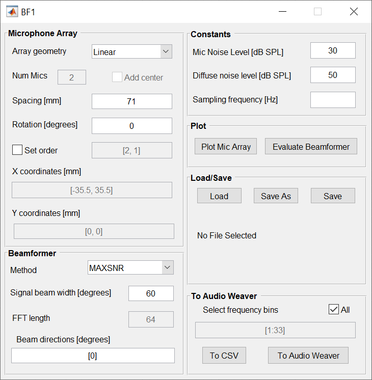
processFunc

Implements a MATLAB version of the module's processing function. This is used by DSP Concepts' regression test framework. It is optional.

getFunc

Similar to the setFunc, but this function is called prior to reading variable information from a module's MATLAB instance structure.

bypassFunc

Implements a custom bypass function when the base class behavior (just copying the input to the output) is not sufficient.

testHarnessFunc

Specifies a MATLAB function which implements a regression test of the module. This is used by DSP Concepts' regression test framework. It is optional.

profileFunc

Used by DSP Concepts' module profiling framework. Optional.

prepareToSaveFunc

This function is called prior to saving a system in Designer. Some modules need to do clean up work before being saved.

Behavior in Designer

This section describes how the modules interact with Designer and how their methods are called at various times.

Dragging Out a Module

When you drag out a module in Designer, it calls the module's constructor function (the _module.m function) with the argument NAME = 'tempName'. The @awe_module object is instantiated and initialized. Upon return, Designer will rename the module. If .defaultName is specified, then it will be used. Otherwise, the module name is generated based on .className.

Changing Module Arguments

After you press to finish editing a module argument, Designer call's your _module.m constructor function with no arguments. This is used to get a list of the arguments.

Next, Designer calls the _module.m function again with the new set of arguments. The new module is instantiated and returned. Call this NEW and the original module OLD.

Designer then uses a generic function to copy module variable values and ranges from OLD to NEW. All previous variable information is copied over. If this does not fit your module, then define a custom .copyVarFunc.

Setting Module Variables

In design mode, if you set a module variable then Designer will update the variable in the MATLAB module instance structure. Then, if the module has a MATLAB .setFunc, it will be called.

In tuning mode, if you set a module variable then Designer will update the variable in the MATLAB module instance structure. Designer will then send a tuning message to the target and update a single variable in the instance structure. Then, if the module has a C Set() function defined, it will be called on the target. If the module does not have a C Set() function but has a MATLAB .setFunc, then the MATLAB .setFunc will be called even in tuning mode.

In both cases, Designer makes sure that the new variable value is within the allowable range. If it falls outside of the range, it will be clipped to the nearest allowable value.

Building the System

During the first part of the build process, Designer is resolving all wire information. This happens in MATLAB. Designer will call your module's preBuildFunc in order to propagate wire information. After the preBuildFunc is called, then your module's MATLAB Set function is called in order to update derived variables. The channel name and channel delay functions will also be called in order to propagate this information.

During the second part of the build process, the module is created on the target. The following steps occur:

1. Designer sends a create_module command which call's the module's C Constructor() function. This allocates memory for the base module instance and initializes all scalar variables (i.e., all non-array variables).

2. The Constructor function then allocates memory for any internal arrays. These are all initially set to zero.

3. After the Constructor returns, the Audio Weaver framework automatically calls the module's set function with mask = 0xFFFFFFFF. At this point, array variables have been allocated but their values have not been set (they are all zero).

4. Next each array variable on the target is initialized by separate tuning messages. This only happens if there is non-zero data in the array. Once an array has been fully initialized, then the module's C Set() function is called with the mask set based on which array variable was written. This repeats N times if the module has N array variables.

Run-time Tuning

When you change a module parameter at run-time, the following interaction with the module occurs.

1. The variable to modify is written by the tuning command (scalar or array variable).

2. If the tuning command is of the "set" variety, then the module's Set() function is called. The MASK value corresponds to the variable that was changed.

3. When you tune via the Designer GUI, then the "set" variety is always used

Deferred Processing

Deferred processing happens at run-time and primarily caused by the ParamSet modules. In the following discussion, the "Controlling" module is the ParamSet while the "Controlled" module is the one whose variables are being modified. The following steps occur:

1. The controlling module writes the variable value of the controlled module directly.

2. The Set function of the Controlled module is called with the mask equal to the macro SETALLMASK. SETALLMASK is defined in fw_Module.h and equals 0xFFFFFF00.

Destroying a System

The system is destroyed when you hit the "Stop" button in the Designer GUI. The following steps occur:

1. Designer sends the "destroy" command to the target.

2. Real-time audio stops.

3. The C Set() function for every module in the system is called with mask = 0. If your module needs clean up operations, like closing a file or freeing memory allocated outside of the Audio Weaver heaps, then do it here.

4. Then all Audio Weaver heaps are freed and reinitialized to zeros.

Loading a System

The stored information on disk contains all of the module arguments and variable values. For each module in your design, Designer will call your module's _module.m constructor function with the stored arguments. Next, it will restore variable values and variable range information.

Parameter Control

This section describes how to get and set variable values from an Audio Weaver system at run-time. There are several core principles that must be understood first before we dive into the control APIs themselves.

1. The Audio Weaver control APIs are designed to write to directly to module instance variables. You can write to scalar variables or to array variables. Updates are made one variable at a time.

2. All variable data types are 32-bits long. Modules can use float, int, uint, and fract32 data types.

3. Modules are identified on the target based on their objectID. Each module has a unique objectID which is set in Designer.

4. Variables within a module are identified based on their offset from the start of the module instance structure. Variable offset values are automatically generated and stored in the module's header file. For example, the file ModScalerDB.h contains:

#define MASK_ScalerDB_gainDB 0x00000100
#define MASK_ScalerDB_gain 0x00000200
#define OFFSET_ScalerDB_gainDB 0x00000008
#define OFFSET_ScalerDB_gain 0x00000009

1. Using the Generate Target Files feature in Designer, you can generate a header file which contains the objectIDs and offsets of all tunable module variables. For each tunable variable, Designer additionally generates a HANDLE which encodes the objectID, offset, coreID, and whether the variable is a scalar or an array.

2. Since you are writing directly to module instance variables, you need to make sure you are writing the proper data type.

3. Audio Weaver does not distinguish between controlling modules during a tuning session (when connected to the Designer PC tools) and controlling modules at run-time in the final deployed system. Similar concepts and APIs are used in both cases.

Assigning objectIDs

You assign objectIDs in Designer on the module's Property View.

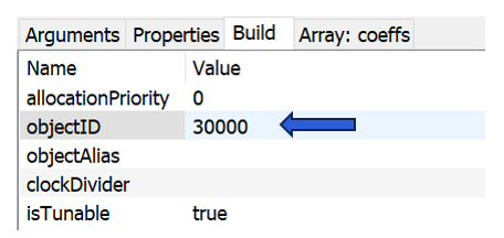
By default, the field "objectID" is empty and the objectID will be automatically assigned when the system is built[^8]. If you want to control the module at run-time, then you should assign a custom objectID. Custom objectIDs are in the range 30000 to 32767.

Generating Target Files

After you have assigned objectIDs in your system, you can generate a header file which is used by your control code. Go to the ToolsGenerate Target Files menu item in Designer. It will open the dialog:

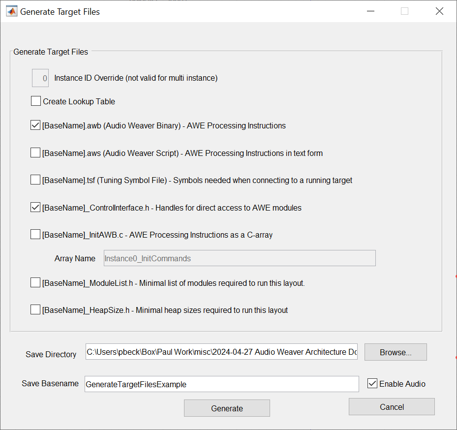
Select "[BaseName]_ControlInterface.h" to generate the handles for your design. Consider the system shown below. 3 modules have assigned objectIDs and these are drawn in bold. You can also see the objectIDs displayed underneath the 3 modules.

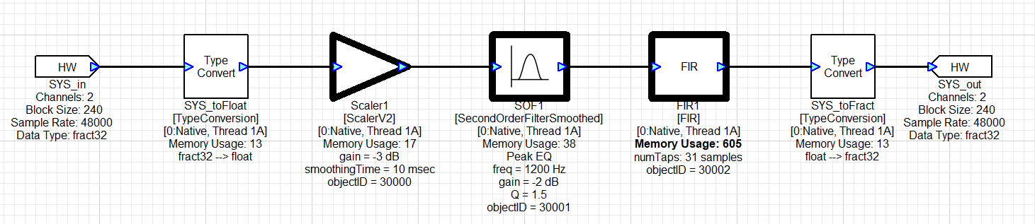
The generated header file contains about 261 lines and provides access to all module variables (parameters, derived, and states). Even hidden variables are included. Here are some of the entries for the Scaler1 module:

#define AWE_Scaler1_classID 0xBEEF0813
#define AWE_Scaler1_ID 30000

// int profileTime - 24.8 fixed point filtered execution time. Must be pumped 1000 times to get to within .1% accuracy
#define AWE_Scaler1_profileTime_HANDLE 0x07530007
#define AWE_Scaler1_profileTime_MASK 0x00000080
#define AWE_Scaler1_profileTime_SIZE 0x00000001

// float gain - Gain in either linear or dB units.
// Default value: 0
// Range: -24 to 24
#define AWE_Scaler1_gain_HANDLE 0x07530008
#define AWE_Scaler1_gain_MASK 0x00000100
#define AWE_Scaler1_gain_SIZE 0x00000001

// float smoothingTime - Time constant of the smoothing process (0 = 
//         unsmoothed).
// Default value: 10
// Range: 0 to 1000
#define AWE_Scaler1_smoothingTime_HANDLE 0x07530009
#define AWE_Scaler1_smoothingTime_MASK 0x00000200
#define AWE_Scaler1_smoothingTime_SIZE 0x00000001

In Process Control APIs

These APIs are used when your control code is running on the same core as the AWECore library you are controlling and your control code shares the same memory space as the audio processing. Examples are a SHARC DSP or an ARM Cortex-M microcontroller. In this case, your control code writes directly into the module instance structure using HANDLEs.

Get/Set a Module Variable

    INT32 awe_ctrlGetValue(const AWEInstance *pAWE, UINT32 handle, void *value, INT32 arrayOffset, UINT32 length)
    INT32 awe_ctrlSetValue(const AWEInstance *pAWE, UINT32 handle, const void *value, INT32 arrayOffset, UINT32 length)

arrayOffset and length are only used when accessing array variables. When accessing scalar variables, you can set these to 0. These functions will automatically call the module's C Get() and Set() functions.

Accessing Module Status (Active, Bypassed, Muted, Inactive)

INT32 awe_ctrlSetStatus(const AWEInstance *pAWE, UINT32 handle, UINT32 status)
INT32 awe_ctrlGetStatus(const AWEInstance *pAWE, UINT32 handle, UINT32 *status)

When accessing a module, you use the handle for any of the module's variables. Internally, the function strips outs the module's objectID.

Getting a Module's Class ID

INT32 awe_ctrlGetModuleClass(const AWEInstance *pAWE, UINT32 handle, UINT32 *pClassID)

This function can be used to check if a module exists, and if so, returns its classID. This can be used to check if the module to control exists on the target and if it is the correct type (class) of module. The generated header file also lists the classID of every controllable module. As in the previous section, this API also uses a variable handle.

Advanced Get/Set Functions

TO-DO: this is all duplicated from the doxygen awecore docs...

The following functions provide finer grained control over how module variables are accessed and are for advanced users. These functions allow you to specify the mask value passed to the module's C Set() and Get() functions and this gives you finer control over when the control functions are called.

    INT32 awe_ctrlSetValueMask(const AWEInstance *pAWE, UINT32 handle, const void *value, INT32 arrayOffset, UINT32 length, UINT32 mask)
    INT32 awe_ctrlGetValueMask(const AWEInstance *pAWE, UINT32 handle, void *value, INT32 arrayOffset, UINT32 length, UINT32 mask)

Control Interface Example

To access a module and control it via the Control Interface,

1. Create the desired layout. In the build tab of a module, assign an objectID to the module's that will be accessed. The objectID must be a value between 30000-32767.

2. Generate a ControlInterface.h header file from the layout with Tools->Generate Target Files. Make sure the [BaseName]_ControlInterface.h box is checked.

3. Include the generated [BaseName]_ControlInterface.h file in the AWE Core integration. This file will contain all of the define's required to use the API's control functions.

4. Check if the module exists and is of the right class with awe_ctrlGetModuleClass().

5. Use one of the awe_ctrl functions to set/get something about a module.

6. The handle, length arguments will all be defined in the [BaseName]_ControlInterface.h file that was generated. See the API Doc for details about the control functions arguments/return values.

7. Check the return value for errors and handle appropriately.

See the following example.

        // Does the current AWE model have a SinkInt module with this control object ID?
        if (awe_ctrlGetModuleClass(&g_AWEInstance, AWE_SinkInt1_value_HANDLE, &classID) == OBJECT_FOUND)
        {
            // Check that module assigned this object ID is of module class SinkInt
            if (classID == AWE_SinkInt1_classID)
            {
                // SinkInt module (value is an array)
                awe_ctrlGetValue(&g_AWEInstance, AWE_SinkInt1_value_HANDLE, &nValue, 0, 1);
            }
        }

TO-DO: this is all duplicated from the doxygen awecore docs...

Remote Control via Tuning Packets

The Audio Weaver Designer GUI and the target processor communicate via the Server as shown in Figure 1. Designer sends text messages over TCP/IP to the Server. The Server converts them to binary message packets, and these are sent to the target processor over the tuning interface. Audio Weaver natively supports tuning over RS232, USB, Ethernet, and SPI.

All messages are originated by Designer or the Server. They are the primary devices in the system. The target processor is the secondary device and only responds to messages. It is a half duplex communication link with the target responding to every message. Only one message can be processed at a time and there is no support for a message queue.

Asynchronous messages generated by the target processor are also not supported. If you need to know something, you'll need to poll for it.

A binary tuning packet consists of an array of 32-bit values and has the structure shown in Figure 35. Every message consists of a header (first word) and a CRC (last word). The message length includes the header and the CRC and thus the shortest message has 2 words. The Core ID is used in multicore systems to route messages to different cores (or instances) of Audio Weaver on the target device. The payload is optional, and the length varies based on the command. The command ID is an 8-bit value and the available messages are defined in the file ProxyIDs.h.

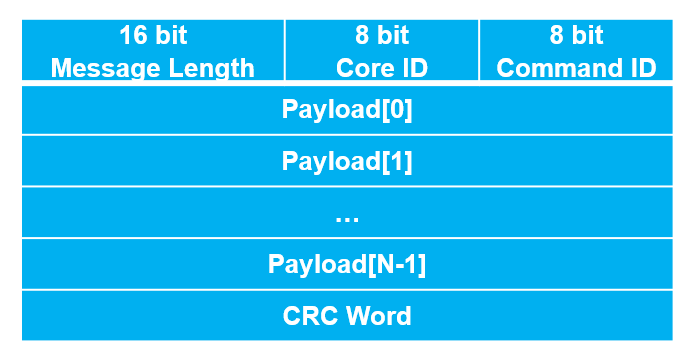
Figure . Binary tuning packet format.

The code below shows how to compute the CRC of a tuning packet.

nLen = packetBuffer[0] >> 16;
UINT32 crc=0;
for(i=0; i < (nLen-1); i++)
{
    crc^=packetBuffer[i];
}

g_PacketBuffer[nLen-1] = crc;

When the Server connects to the target processor it reads back the length of the tuning buffer. This sets the maximum message length that can be sent to the target and is enforced by the Server. Refer to Figure 7 and note that the "Communication buffer size" is listed as 264 words. This is the minimum recommended size and the small size is due to the need to save memory on deeply embedded DSPs and microcontrollers.

The tuning messages are executed in the Deferred Processing Thread mentioned in Section 3.4. This thread executes at a lower priority compared to any of the real-time audio processing threads. Thus, the tuning messages will not interfere with real-time audio.

The full set of tuning messages is documented on the DSP Concepts website. The vast majority are used internally by Designer. A few messages are useful for run-time control and we focus on these.

PFID_SetValue

This message writes a scalar variable and does not call the module's Set() function.

Message Length = 5	coreID	PFID_SetValue
uint address
int/float/fract32 value
uint offset
uint CRC

The address combines the objectID of the module and the variable offset as follows:

address = (objectID << 12) + offset;

Alternatively, you can calculate the address using the variable's HANDLE (see Section 5.2) as:

address = handle & 0x3ffff07f;

After the command is executed on the target, it sends the following 2 word reply packet:

Error status

---

CRC

This is the standard reply for messages that do not have a payload. You should check that Error Status == E_SUCCESS to verify that the operation was successful. Common errors could be an incorrect address or non-existing coreID. The entire list of error codes is found in Errors.h.

PFID_SetValueSetCall

This message writes a scalar variable and calls the module's Set() function with a specified mask.

Message Length = 6	coreID	PFID_SetValueSetCall
uint address
int/float/fract32 value
uint mask
uint offset
uint CRC

The mask comes out of the generated target files described in Section 5.2. The standard reply is returned.

PFID_SetValues

Writes an array of numWords values and does not call the module's Set() function.

Message Length = 5 + numWords	coreID	PFID_SetValues
uint address
uint offset
uint num words to write
int/float/fract value 1
int/float/fractvalue 2
…
int/float/fractvalue N
uint CRC

The standard reply is returned.

PFID_SetValuesSetCall

Writes an array of numWords values and does call the module's Set() function.

Message Length = 6 + argCount	coreID	PFID_SetValuesSetCall
uint address
uint offset
uint mask
uint argCount
int/float/fract32 val1
....
uint CRC

The standard reply is returned.

PFID_FetchValue

Reads a scalar value from the target. Does not call the module's Get() function.

Message Length = 4	coreID	PFID_FetchValue
uint address
uint offset
uint CRC

The reply packet contains 4 words:

Message Length = 4	0
int error status
int/float/fract32 value
uint CRC

PFID_GetCallFetchValue

Reads a scalar value from the target and call's the module's Get() function before the read is performed.

Message Length = 5	coreID	PFID_GetCallFetchValue
uint address
uint mask
uint offset
uint CRC

The reply packet is the same as the one for PFID_FetchValue.

PFID_FetchValues

Reads an array of numWords from the target. Does not call the module's Get() function.

Message Length = 5	coreID	PFID_FetchValues
uint address
uint offset
uint num words to read
uint CRC

The reply packet is:

Message Length = 3 + numWords	0
int error status
int/float/fract value 1
int/float/fractvalue 2
…
int/float/fractvalue N
uint CRC

PFID_GetCallFetchValues

Reads an array of numWords from the target and calls the module's Get() function before the read is performed.

Message Length = 6	coreID	PFID_GetCallFetchValues
uint address
uint offset
uint mask
uint words to read
uint CRC

The reply packet is the same as PFID_FetchValues.

MASK Usage Guidelines

The previous section presented a total of 8 different tuning commands. They covered:

(Set + Get) x (Scaler + Array) x (No-MASK + MASK)

That is a lot of combinations and what is the best way to use the MASK? The safest thing is to always use the MASK when setting or getting values. The only exception is when writing or reading long arrays that exceed the length of the message buffer. For example, suppose that you are writing a 1024 word array. Looking at SetValues, we see that the message length is 5 + numWords. And for SetValuesSetMask the message length is 6+numWords. If the message buffer is 264 words long, then the longest message you can send is about 256 words. To write an array with 1024 words, you'll send 4 subarrays and only set the MASK on the last write. The module's Set() function is called only after the array has been completely updated.

SetValues [0 to 255]

SetValues [256 to 511]

SetValues [512 to 767]

SetValuesSetMask [768 to 1023]

Controlling Audio Processing on an SOC

Modern SOCs have multiple processors. Some are running a high-level OS (HLOS) like Linux or Android. The audio processing happens on dedicated DSPs or leverages an Arm core. The control code typically runs on the HLOS and needs to control processing on another core. This means that the In-Process Control APIs described in Section 5.3 will not work. To solve this, Audio Weaver leverages the tuning packet approach of Section 5.4. In the final system, you need the ability to simultaneously tune the system and control it from the HLOS. The design used is shown in Figure 36. All control is funneled through an AWEController service. Tuning messages from the PC arrive over TCP/IP and local control is via the Audio Manager. The AWEController sends the messages through shared memory to the DSP and collects the reply packets. The AWEController serializes the messages so that only one message is active at a time.

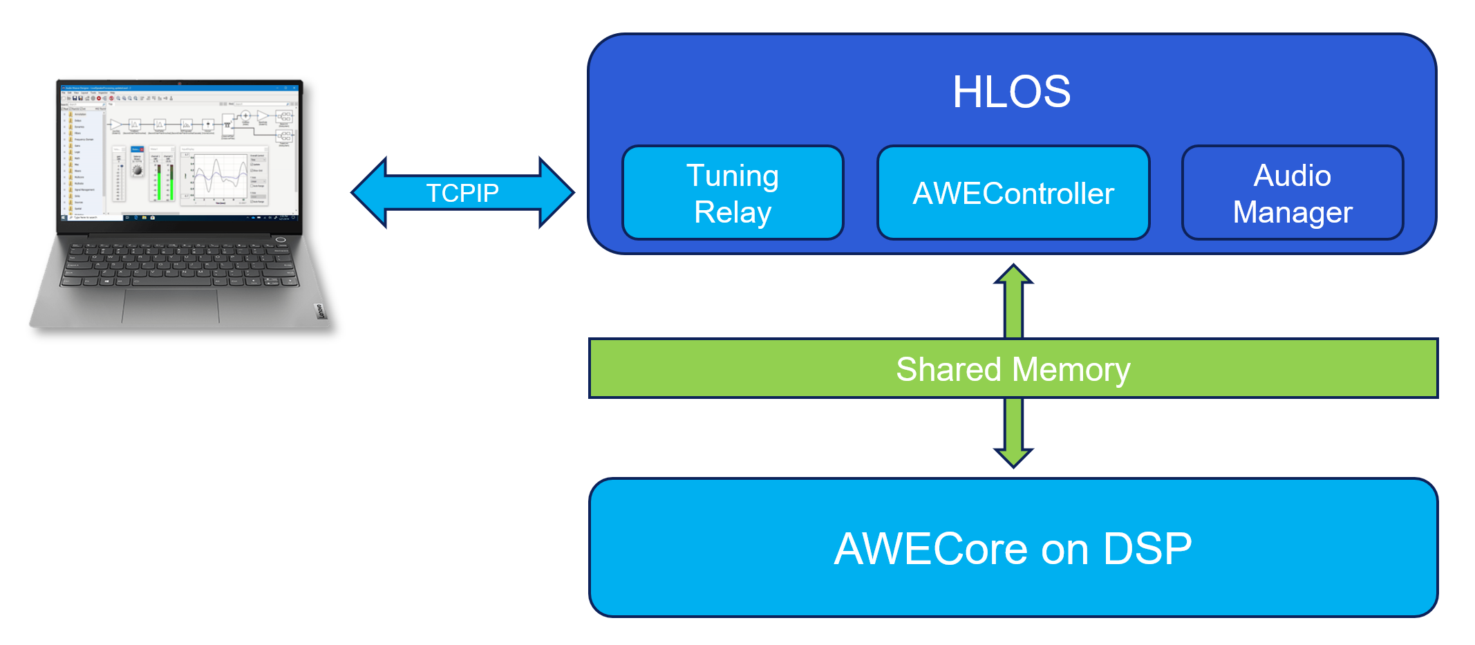
Figure . HLOS control using an AWEController service which manages communication with the DSP via shared memory.

Threading Considerations for Parameter Control

Real-time audio processing and control happen in different software threads in Audio Weaver. Control is usually at a lower priority and is pre-empted by real-time processing. However, on processors like the Hexagon which have multiple hardware threads, the control code and the audio processing can occur at the same time.

The control thread writes module instance variables and calls the module's C Set() function. You have to write your module code to take into account this pre-emption and design your module in a way that it is robust. Let's consider how to properly implement a Biquad filter so that coefficient updates do not lead to filter instability.

The first array you add to your module are the user tunable coefficients. This is a parameter.

add_array(M, 'coeffs', 'float', [1; 0; 0; 0; 0], 'parameter','[b0; b1; b2; a1; a2]');

Then add another set of filter coefficients and mark them as derived.

add_array(M, 'coeffsProc', 'float', [1; 0; 0; 0; 0], 'derived', '[b0; b1; b2; a1; a2]');

These coefficients will be used by the module's processing function. Then define a C Set() function for the module. The set function will swap coefficient pointers whenever the .coeffs array is updated.

UINT32 awe_modBiquadSet(void *pInstance, UINT32 mask)
{
    awe_modBiquadInstance *S;
    FLOAT32 tempPtr;
    if (mask & MASK_Biquad_coeffs)
    {
        tempPtr = S->coeffsProc;
        S->coeffsProc = S->coeffs;
        S->coeffs = tempPtr;
    }

    return 0;
}

This is just one of many possible approaches to solving this problem.

Custom Control Packets

In some cases, you want your module to accept a "control packet" and modify multiple instance variables at the same time. Or you may want to obfuscate the tunable variables in your module. To accomplish this, add an array variable to your design which can be used to exchange the custom control packets with your tuning tools:

add_array(M, 'controlPacket', 'float', zeros(1024, 1), 'parameter', 'Used by custom tuning tools');

You can size this array, as needed by your algorithm. Your tuning tools can read/write this array and your module's Get() and Set() functions can interpret the payload.

The main downside of this approach is that the module can no longer be easily controlled via the Designer GUI.

Best Practices Using Control Arrays

A typical automotive system has 20 to 30 modules which need to be controlled at run-time. One possible approach to designing the control interface is to assign objectIDs to each of these modules and generate target files as discussed in Section 5.2. This is a fine approach, but the main downside is that every time you change your control API, you'll need to generate a target file and rebuild the Audio Manager on the HLOS.

An alternate approach is to aggregate all controllable parameters into a single SourceInt module. This module holds an array of N values and has an objectID assigned to it. Then, you would extract individual values out of this array and write them into specific module variables using the MapperControl and ParamSet modules. The advantage of this approach is that you would have to expose only a single objectID and can make changes to the control code via changes to the Audio Weaver signal flow. Plus, if your design has 40 tunable variables, oversize the control array to 50 values. This gives you expansion in the future. This is the recommended approach when controlling large signal flows, like automotive systems.

An example of using a control array is shown in Figure 37. This shows a portion of the top-level system and you'll notice that there is a SourceInt module called "Control_IPC_In" to which the HLOS writes and a SinkInt module called "Control-IPC_Out" that can be read by the HLOS.

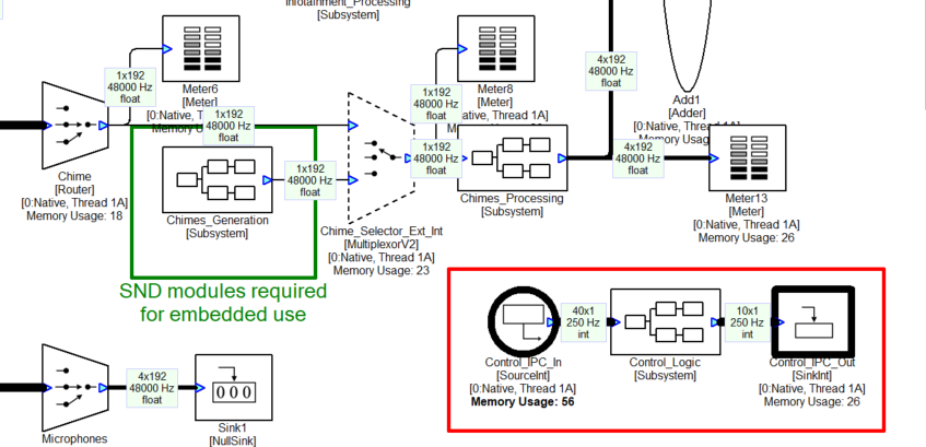
Figure . Portion of an automotive signal flow which shows consolidated control via SourceInt and SinkInt modules.

Inside the Control_Logic subsystem are multiple ParamSet modules which write into various modules. For example, the control array has 3 values for controlling the Bass, Mid, and Treble tone controls. The MapperControl module extracts one of the 3 values (channelNum as shown on the inspector), clips input values to the range [0 20], and then remaps linearly to the dB range of [-10 +10]. This is then fed into a ParamSet module which writes the value into another module.

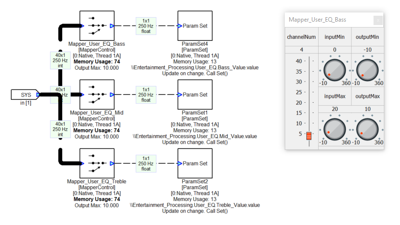
Tuning Relays

Figure 1 shows the high-level Audio Weaver architecture. The Server talks directly to the target hardware via one of the standard tuning interfaces supplied with Audio Weaver. There are times when none of the standard tuning interfaces are suitable, and you need to tunnel messages using a custom protocol. The solution is to use a Tuning Relay.

A Tuning Relay is a custom application which sits between the Server and your target as shown in Figure 38. The tuning relay can run under Windows or on an applications processor of your SOC. To the Server, the tuning relay looks like a TCP/IP target. The tuning relay receives messages from the Server, repackages and sends them over the custom interface. The tuning interfaces translates both transmit and receive messages.

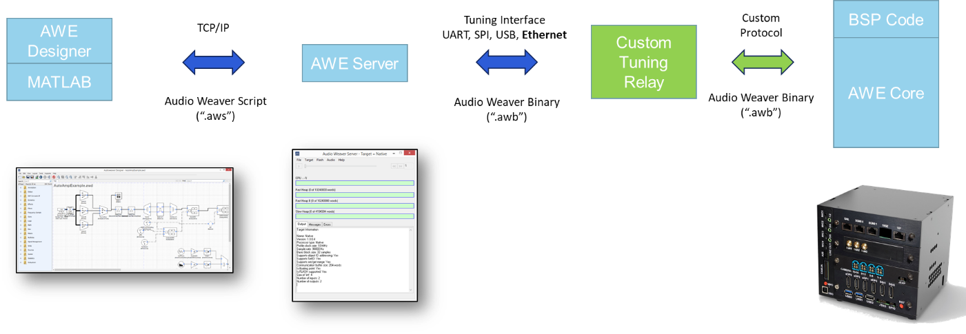
Figure . Custom tuning relay is used to send tuning messages via a custom protocol.

MATLAB API

This section describes Audio Weaver's MATLAB automation API. It allows you to leverage the power of MATLAB to configure and control Audio Weaver. The API can be used for parameter calculation, visualization, general automation, regression tests, and even full system design. The API is an advanced feature and assumes that the user is familiar with MATLAB.

The most straightforward use of the API allows MATLAB to interact with the Audio Weaver Designer GUI. This is the focus of this Section and is sufficient for most users. More advanced scripting features including the full API are separately described in the document Audio-Weaver---MATLAB-API.

MATLAB is an interpreted scripting language and all of the commands shown in this section can be typed in directly into MATLAB.

Requirements

The API is compatible with MATLAB version 2021b or later. You'll need a standard MATLAB license and the Signal Processing Toolbox. The MATLAB API is included with the "Pro" versions of Audio Weaver; it is not part of the Standard version.

Setup

After installing Audio Weaver Developer or Pro, update MATLAB's search path to include the directory:

matlab

where represents the installation directory. This directory contains the primary set of MATLAB scripts used by the tool. Note that you only have to add a single directory to the MATLAB path and not all of the subdirectories recursively. The MATLAB menu item "File Setup Path..." can be used to update the path. Once the path is set, issue the command:

awe_designer

This launches the Audio Weaver Server followed by the Designer application. It also configures additional directories and initializes global variables. If you just want to launch the Server and configure MATLAB to run scripts, then simply execute

awe_init

If you accidentally shut down the Server while using Audio Weaver Designer, then press the Reconnect to Server button found on the toolbar.

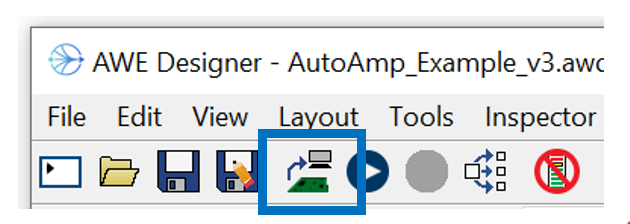
If you are not using Designer, then you can reconnect to the Server by reissuing the awe_init command.

On-line help

All of the Audio Weaver MATLAB functions have usage instructions within the function header. To get help on a particular function, type

help function_name

Additional help is available for audio modules. The command

awe_help

creates a list of available audio modules in the MATLAB command window. A partial list is shown below:

awe_help

GPIO_module - Misc

abs_fract32_module - BasicAudioFract32

abs_module - BasicAudioFloat32

acos_module - MathFloat32

adder_fract32_module - BasicAudioFract32

adder_int_module - BasicInt32

adder_module - BasicAudioFloat32

agc_attack_release_fract32_module - BasicAudioFract32

Each of the modules appears as a hyperlink, and clicking on an item provides detailed module specific help. The help provided is above and beyond the comments shown in the file header and accessed via the standard MATLAB "help" command. You can also obtain help for a specific module using the MATLAB command line. For example, to get help on the FIR filter module, type:

awe_help fir_module

Manipulating Parameters

The most basic way of using the MATLAB API is to get and set parameters in a system that is loaded in Audio Weaver Designer. Assume that you have the system "Example1.awd" open in Designer.

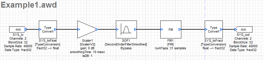
Then from the MATLAB prompt, type

GSYS = get_gsys('Example1.awd');

This returns a MATLAB structure which contains the entire state of the Designer GUI[^9]. We won't go into the details here; the only item of interest is the field .SYS which we call the system structure

GSYS.SYS = NewClass // Newly created subsystem
    SYS_toFloat: [TypeConversion]
    Scaler1: [ScalerV2]
    SOF1: [SecondOrderFilterSmoothed]
    FIR1: [FIR]
    SYS_toFract: [TypeConversion]

The system structure contains one entry per module in the system. Looking more closely at Scaler1 we see all of the internal parameters of the module:

GSYS.SYS.Scaler1

Scaler1 = ScalerV2 // General purpose scaler with a single gain

gain: 0 [dB] // Gain in either linear or dB units.

smoothingTime: 10 [msec] // Time constant of the smoothing process.

isDB: 1 // Selects between linear (=0) and dB (=1) operation

The first line displays 3 items:

"Scaler1" -- the name of the module within the system.

"ScalerV2" -- the underlying class name or type of the module.

"General purpose scaler ..." -- this is a short description of the function of the module.

The next three lines list exposed interface variables that the module contains. A variable may display applicable units in brackets (e.g, [msec]) and have a short description.

To change the gain of the module, type

GSYS.SYS.Scaler1.gain = -6;

The gain change occurs locally in the MATLAB environment and also in Designer. You will see the changed variable when you reopen the inspector for Scaler1 or redraw the canvas[^10]. If the system in Designer is built and running, then the gain change will also occur on the target processor when it is changed in MATLAB.

Commonly Used Commands

This section describes commonly used MATLAB commands.

Showing Hidden Variables

By default, the MATLAB API does not show hidden variables (e.g., filter state variables). If you would like to make these visible, type

global AWE_INFO;
AWE_INFO.displayControl.showHidden = 1;

AWE_INFO is a global variable which controls various aspects of Audio Weaver. The standard view of the SecondOrderFilterSmoothed module is

GSYS.SYS.SOF1
    SOF1 = SecondOrderFilterSmoothed // General 2nd order filter designerwith smoothing
    filterType: 0 // Selects the type of filter that is implemented.
    freq: 250 [Hz] // Cutoff frequency of the filter, in Hz.
    gain: 0 [dB] // Amount of boost or cut to apply, in dB if applicable.
    Q: 1 // Specifies the Q of the filter, if applicable.
    smoothingTime: 10 [msec] // Time constant of the smoothing process.

And now with hidden variables shown

GSYS.SYS.SOF1
SOF1 = SecondOrderFilterSmoothed // General 2nd order filter designer
with smoothing
filterType: 0 // Selects the type of filter that is implemented.
freq: 250 [Hz] // Cutoff frequency of the filter, in Hz.
gain: 0 [dB] // Amount of boost or cut to apply, in dB if applicable.
Q: 1 // Specifies the Q of the filter, if applicable.
smoothingTime: 10 [msec] // Time constant of the smoothing process.
updateActive: 1 // Specifies whether the filter coefficients are updating
b0: 1 // Desired first numerator coefficient.
b1: 0 // Desired second numerator coefficient.
b2: 0 // Desired third numerator coefficient.
a1: 0 // Desired second denominator coefficient.
a2: 0 // Desired third denominator coefficient.
current_b0: 1 // Instantaneous first numerator coefficient.
current_b1: 0 // Instantaneous second numerator coefficient.
current_b2: 0 // Instantaneous third numerator coefficient.
current_a1: 0 // Instantaneous second denominator coefficient.
current_a2: 0 // Instantaneous third denominator coefficient.
smoothingCoeff: 0.064493 // Smoothing coefficient. This is computed based on the smoothingTime, sample rate, and block size of the module.
state: [2x2 float] // State variables. 2 per channel.

You'll now see derived variables and state variables which are normally hidden from view.

Building Systems

If the system in Audio Weaver Designer is in Design mode, you can build the system using

GSYS = get_gsys('Example1.awd');
GSYS.SYS = build(GSYS.SYS);

and then you can start real-time audio playback with

test_start_audio;

Loading and Saving Designs

Instead of loading the GSYS structure from Designer, you can load it directly from disk

GSYS = load_awd('Example1.awd');

Then when you are done making modifications, save it to disk

save_awd('Example1.awd', GSYS);

Variable Ranges

Audio Weaver variables can have range information associated with them. To view a variables range information, you can type

GSYS.SYS.Scaler1.gain.range

ans =

-24 24

If you try and set a value outside of the allowable range then a warning will occur:

GSYS.SYS.Scaler1.gain = -40;

Warning: Assignment to variable gain is out of range. Value: -40. Range: [-24:24]

In awe_variable_subsasgn at 64

In awe_module.subsasgn at 86

In awe_module.subsasgn at 128

To change the range of a variable, simply update the .range field

GSYS.SYS.Scaler1.gain.range = [-50 0];

Advanced Features with MATLAB

This section merely touched upon the power of the MATLAB automation API. The API is also used for:

1. Module regression testing

2. Automated profiling

3. Script based design of subsystems

4. Creating custom modules

5. Custom inspectors

6. Batch processing of files. On PC and on target

7. Generating preset files

8. Creating target files in an automated fashion

Integrating Audio Weaver Into Products

To build a product with Audio Weaver technology, you have to integrate the Audio Weaver run-time library into your codebase. The Audio Weaver library essentially processes blocks of audio data while your code needs to manage audio I/O and interrupts. We refer to the code outside of Audio Weaver as the board support package (BSP). This section begins with general principles around an Audio Weaver BSP integration. We then describe the AWECore API used in deeply embedded processors like microcontrollers and DSPs. Finally, we describe the differences in the AWECore OS APIs used in high-level operating systems.

General Principles

The AWECore run-time library has 5 main APIs:

1. Initialize the Audio Weaver instance structure.

2. Initialize the signal flow.

3. Pass blocks of real-time audio data into and out of the library. This is handled with real-time threads.

4. Service the tuning interface. This runs at a lower priority to the real-time audio threads.

5. Service the deferred processing. This runs at a lower priority to the real-time audio threads.

Audio I/O and the tuning interface require responding to interrupts (or callbacks). You can write this BSP code "bare metal" and manage interrupts yourself or leverage a real-time operating system for scheduling and priorities.

The highest priority interrupt in the system is for audio I/O at the basic block size as described in Section 3.1.1. This is the smallest block size of the system and usually corresponds to the DMA buffer size. Your system will also require additional lower priority threads for multithreaded processing. We recommend at least 3 other audio threads.

You will also need a lower priority thread to perform deferred processing as described in Section 3.4. This thread responds to tuning messages and handles module control functions.

Instance Initialization

The AWECore instance structure holds the entire state of the Audio Weaver system. This instance structure is of type AWEInstance. The instance structure is initialized once at system start up and you specify:

• Memory heaps and sizes

• Hardware input and output pin properties

• Tuning buffer memory and size

• Module table

• Target information. See Section 2.1.10

• Callback functions to start and stop audio

After the structure has been initialized by your code, you call the API:

INT32 awe_init(AWEInstance *pAWE);

Audio Weaver manages its own set of 3 or 4 heaps and you pass in pointers to the heap memory sections when initializing the AWECore instance. We recommend statically initializing this memory in deeply embedded systems, or mallocing this memory if you have a high-level OS. The type of memory assigned to the heaps has a large impact on overall processing efficiency. We recommend using internal or tightly coupled memory for the FAST heaps. External SDRAM or DDR is suitable for the SLOW_HEAP[^11].

An Audio Weaver run-time image is built with a set of included audio modules. This is specified through a macro during the compilation process. Reducing the number of audio modules allows you to reduce the memory footprint of Audio Weaver. This is important in deeply embedded systems but not that important with Linux or Android based systems.

More details of this initialization process and example code can be found here. Once initialized, the instance structure is used by all other APIs.

Loading the Signal Flow

After the AWECore instance is initialized, it does not contain a signal flow. It is similar to an empty canvas shown in Designer. A signal flow in Audio Weaver is initialized via a series of AWB commands. When you are connected to the PC, these commands are received over the tuning interface. When you are running standalone, the AWB information must be stored locally. This can be done two different ways from the Generate Target Files dialog discussed in Section 5.2.

InitAWB.c

Recall that the tuning messages are all arrays of 32-bit integers. The first option turns the tuning messages into an initialized C array of data.

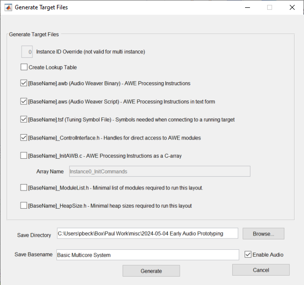
You add this static C array to your project and recompile. This is useful for deeply embedded processors that do not have a file system.

Then in your code you call this function to load the AWB information and initialize the signal flow:

INT32 err = awe_loadAWBfromArray (&g_AWEInstance, pCommands, arraySize, &nErrOffset);

if (err)
{
    // report the error
    printf("error code %u due to command at position %un", err, nErrOffset);
    // handle the error
    ...
}

where

pCommands is a pointer to the array of AWB data

arraySize is the length of the array, in words.

nErrOffset is used for error reporting. If the load fails then nErrOffset will contain the array offset of the failing message.

The returned errors are defined in the file Errors.h.

AWB File

The second option creates a binary file with an .awb extension. This is useful if your product has a file system.

In your application code, you would fread() the binary data into an internal array and then call the awe_loadAWBFromArray() function[^12].

Presets

AWB files created via Generate Target Files contain the entire signal flow. It is possible to generate AWB files which only contain parameters writes. We refer to these as Preset Files. You can store preset files in your final product and load them at run-time. Preset files are useful for changing a large number of parameters simultaneously in your system, more than can be comfortably managed via the control APIs. In automotive systems, preset files are frequently used for different sounds modes.

The best way to generate preset files is to leverage the MATLAB Automation API described in Section 6. Alternatively, you can also manually generate them via custom tuning tools.

Real-time Audio I/O

During initialization, you will configure your real-time audio I/O and create threads needed for processing. Then in the interrupt handler for the basic block size (the high priority interrupt), you will:

1. Copy data from your input peripherals into the Audio Weaver Hardware Input Pin. For each channel of audio call the function:

INT32 awe_audioImportSamples(const AWEInstance * pAWE, const void * inSamples, INT32 inStride, INT32 channel, SampleType inType)

This copies the audio data from inSamples into the input wire buffer of your signal flow. The data is copied into the specified channel number. inStride is the stride between input samples and inType specifies whether the input data is 16-, 24-, or 32-bits long. All input and output samples are fixed-point.

1. Copy data from the Audio Weaver signal flow into your output peripherals. For each channel of audio call the function:

INT32 awe_audioExportSamples(const AWEInstance *pAWE, void *outSamples, INT32 outStride, INT32 channel, SampleType outType)

This copies the data from Audio Weaver into the outSamples buffer. Data is read from the specified channel. The function increments the write pointer by outStride after writing each audio sample. outType specifies the format of the destination audio samples.

1. The final step in the audio ISR is to determine which audio processing thread can execute. That is, which audio thread has enough data to process. First call the function:

layoutMask= awe_audioGetPumpMask(&g_AWEInstance);

This returns a bitmask specifying which audio threads can run with the LSB corresponding to the highest priority thread. You would check these bits and then raise interrupts as shown next. If your system supports N audio threads, then you would repeat this process for all N low order bits.

// Within the ISR
if (layoutMask & 0x1) raise(AWEProcess_HiPrio);
if (layoutMask & 0x2) raise(AWEProcess_LowPrio);

// ISR handlers
AWEProcess_HiPrio()
{
    awe_audioPump(&g_AWEInstance, 0); // small block size path
}

AWEProcess_LowPrio()
{
    awe_audioPump(&g_AWEInstance, 1); // large block size path
}

The design above is the easiest to implement and performs all audio processing in lower priority worker threads. If you need extremely low latency (such as for road noise cancellation), then the processing of the basic block size happens in the ISR and the code changes slightly as shown below.

// Import all input audio data
layoutMask= awe_audioGetPumpMask(&g_AWEInstance);
if (layoutMask & 0x1)
{
    // Pump the smallest block size in ISR
    awe_audioPump(&g_AWEInstance, 0);
}

// Raise user interrupt for lower priority thread
if (layoutMask & 0x2) raise(AWEProcess_LowPrio);
// Export all output audio data

The real-time audio architecture in Audio Weaver assumes that all I/O is synchronized. This requires all audio devices to be on the same clock. If you have multiple clocks, then we recommend using an asynchronous sample rate converter (ASRC) with your BSP code at the input or output of your system. DSP Concepts has a software ASRC library that can be used, if needed.

Tuning Interface

The tuning interface revolves around a global array of 32-bit values called the Packet Buffer. A pointer to the packet buffer is provided to the AWEInstance structure during initialization together with the packet buffer length. You would write custom code for receiving tuning messages from the PC via the selected tuning interface and you would write the data into the Packet Buffer. Pseudo code is shown below.

// At AWEInstance initialization time

#define PACKET_BUFFER_SIZE 264
UINT32 AWE_Packet_Buffer[PACKET_BUFFER_SIZE];
g_AWEInstance.packetBufferSize = PACKET_BUFFER_SIZE;
g_AWEInstance.pPacketBuffer = AWE_Packet_Buffer;

// Then in the callback which receives tuning messages
// write the received message directly into AWE_Packet_Buffer

// This is your custom code
readPacket(&AWE_Packet_Buffer, sizeOfPacket);

// This Audio Weaver function executes the message and generates a reply
// inplace in the AWE_Packet_Buffer.

awe_packetProcess(&g_AWEInstance);

// Now send the reply message back to the PC.

// This is your custom code
writePacket(&AWE_Packet_Buffer_Reply, sizeOfPacket);

You have to ensure that the call to awe_packetProcess() occurs at a lower priority than any audio processing threads.

The speed of the tuning experience is critical to the usability and agility of Audio Weaver. We recommend that your tuning implementation can process at least 200 tuning messages per second from the Designer tools. You can use the Tuning Interface Speed Test described in Section 2.1.12.2 to verify the performance of your implementation.

Deferred Processing

This thread manages housekeeping operations for audio modules. The firmware author can check for any required deferred processing using the return value of awe_audioPump(), which will return TRUE if any deferred processing is pending. If deferred processing is needed, then call awe_deferredSetCall() at a priority that is lower than the audio processing.

awe_deferredSetCall() performs deferred processing for a single module, and returns TRUE if there is more deferred processing that is pending. Thus, it should be called repeatedly until it returns FALSE.

//g_bDeferredProcessingRequired is returned by awe_audioPump()

if (g_bDeferredProcessingRequired || bMoreProcessingRequired)
{
    g_bDeferredProcessingRequired = FALSE;
    bMoreProcessingRequired = awe_deferredSetCall(&g_AWEInstance);
}

Testing your BSP

Audio Weaver Designer can be used to verify the implementation of a BSP. There are Audio Weaver modules for stressing the CPU load and memory bandwidth of the system. Plus, Designer has integrated tests of the tuning interface. At a minimum, you should verify that:

1. Tuning interface is robust and achieves at least 200 messages per second.

2. System is glitch free even with high CPU load (> 95%)

3. Tuning interface works during high CPU load

4. All audio I/O is glitch free and you have constant repeatable latency between audio devices even between system reboots.

5. Deferred processing and tuning messages are handled in a lower priority thread and do not lead to audio pops and click

You can do even deeper system validation with DSP Concepts Real Time Audio System Check (RTASC). This is a guided step-by-step procedure for measuring the performance of your audio system. Besides the BSP checks, it also verifies:

1. Microphone noise floor

2. Microphone sensitivity including matching between mics

3. Microphone isolation (to ensure correct porting and sealing)

4. Loudspeaker THD

5. Conducted sound between speakers and microphones

We recommend running RTASC before tuning and voice enabled products

Changes for AWECore OS Deployments

The AWE Core library is designed to be portable across many different processor types and runs "bare metal" without access to an operating systems. AWECore OS, on the other hand, is designed for Linux and Android usage, and leverages the operating system for File I/O, TCP/IP Sockets, and multi-threading. Using native components of AWECore OS, users can easily load layouts from AWBs, record input and output audio streams, process and log TCP/IP tuning command packets, and run complex, multi-threaded signal processing flows across multiple cores.

[^1]: Requires MATLAB 2021b or later and the Signal Processing Toolbox.

[^2]: The module DLLs are stored in the same directory as the Server executable. If you write your own custom modules, then you would place your DLL into this directory.

[^3]: The limiting factor is cache size in SOCs. For larger block sizes, the processing may become less efficient if there are many cache misses.

[^4]: An audio module can specify if it supports in-place processing or requires distinct input and output wire buffers. If it supports in-place, then Audio Weaver will try and reuse the same wire buffers. This is not always possible based on the system topology. If the module requires distinct buffers, then this will always be provided.

[^5]: Very similar to how custom effects are loaded by digital audio workstations.

[^6]: This is a deprecated module, but is used as an example since it is easy to understand.

[^7]: The terminology "single heap" was before the days of the SHARED HEAP. The single heap design combines the first 3 heaps and actually still includes the SHARED heap.

[^8]: Wires, modules, and layouts are all assigned objectIDs at build time. They are sequentially numbered starting at 1. If you assign a custom objectID, then the sequentially generated value will be overwritten at build time.

[^9]: More specifically, it returns a pointer to a global structure which holds the state of Designer.

[^10]: Prior to Audio Weaver 8.D.2.5, changes made in Matlab weren't immediately reflected in Designer. You had to send the updated GSYS.SYS structure back to Designer using the command set_gsys(GSYS, 'Example1.awd').

[^11]: Audio Weaver also supports a single heap if your processor has only a single type of memory available.

[^12]: The AWECore OS APIs described later can load and process the AWB file information directly from disk.